{
"cells": [
{
"cell_type": "markdown",
"id": "89c0718d-5af1-475f-a0f1-d2be04397808",
"metadata": {},
"source": [
"# NumPy for Linear Algebra\n",
"\n",
"Created by Ben Poole, Summer 2024\n",
"\n",
"Edited by Razvan Bunescu, Fall 2024"
]
},
{
"cell_type": "markdown",
"id": "9ca4c94c-5304-4e71-83fa-5f8dc86c820f",
"metadata": {},
"source": [
"## Table of Notation\n",
"\n",
"$\n",
"\\newcommand{\\xv}{\\mathbf{x}}\n",
"\\newcommand{\\wv}{\\mathbf{w}}\n",
"\\newcommand{\\yv}{\\mathbf{y}}\n",
"\\newcommand{\\tv}{\\mathbf{t}}\n",
"\\newcommand{\\zv}{\\mathbf{z}}\n",
"\\newcommand{\\uv}{\\mathbf{u}}\n",
"\\newcommand{\\vv}{\\mathbf{v}}\n",
"\\newcommand{\\bv}{\\mathbf{b}}\n",
"\\newcommand{\\av}{\\mathbf{a}}\n",
"\\newcommand{\\R}{\\rm I\\!R}\n",
"\\newcommand{\\sign}{\\text{sign}}\n",
"\\newcommand{\\Ym}{\\mathbf{Y}}\n",
"\\newcommand{\\Tm}{\\mathbf{T}}\n",
"\\newcommand{\\Xm}{\\mathbf{X}}\n",
"\\newcommand{\\Wm}{\\mathbf{W}}\n",
"\\newcommand{\\Zm}{\\mathbf{Z}}\n",
"\\newcommand{\\Um}{\\mathbf{U}}\n",
"\\newcommand{\\Vm}{\\mathbf{V}}\n",
"\\newcommand{\\Am}{\\mathbf{A}}\n",
"\\newcommand{\\muv}{\\boldsymbol\\mu}\n",
"\\newcommand{\\Sigmav}{\\boldsymbol\\Sigma}\n",
"\\newcommand{\\Lambdav}{\\boldsymbol\\Lambda}\n",
"$\n",
"\n",
"\n",
"| Symbol | Meaning | Symbol | Meaning |\n",
"|-----------------------|-------------------------------|-----------------------------------------------------|--------------------------------|\n",
"| $D$ | dataset | $h$
$f$ | hypothesis function |\n",
"| $\\Xm$ | input / data matrix | $x_{i,j}$ | $i$th row and $j$th column |\n",
"| $\\xv$
$\\vec{x}$ | feature / input vector | $x_i$ | $i$th element |\n",
"| $\\Ym$
$\\Tm$ | labels / targets matrix | $\\yv$
$\\tv$ | labels/targets vector |\n",
"| $N$ | number of features / columns | $M$ | number of data samples / rows |\n",
"| $(\\xv, \\yv)$ | training sample | $(\\xv', \\yv')$ | testing sample |\n",
"| | | $\\hat{\\yv}$
$f(\\xv {;} \\wv)$
$h(\\xv {;} \\wv)$ | predictions "
]
},
{
"cell_type": "markdown",
"id": "674201a9-99c5-4424-82b8-483164e900fa",
"metadata": {},
"source": [
"# NumPy Review\n",
"\n",
"NumPy is a scientific library that is frequently used for its highly optimized linear algebra powers. One of NumPy's main attractions is its N-dimensional array objects which work great for storing and manipulating datasets! As we will come to see, most datasets are just 2D arrays where the number of data samples corresponds to the number of rows and the number of features corresponds to the number of columns. "
]
},
{
"cell_type": "code",
"execution_count": 1,
"id": "c6494bff-ea2c-43d9-8a04-ae4c61231794",
"metadata": {},
"outputs": [],
"source": [
"import traceback\n",
"import numpy as np\n",
"\n",
"# Sets NumPy gloabl seed such that any\n",
"# randomly generation done by NumPy is seeded\n",
"np.random.seed(0)"
]
},
{
"cell_type": "markdown",
"id": "46b01904-6566-4bb2-b34d-85f62d211511",
"metadata": {},
"source": [
"## Generating Arrays\n",
"\n",
"A numpy array is a grid of values, typically all of the same type. Array values can be indexed by either a integer or tuple/list of nonnegative integers. The number of dimensions is usually referred to as the rank of the array; the shape of an array is a tuple of integers giving the size of the array along each dimension [1].\n",
"\n",
"Let's make this definition concrete by first creating a rank 1 array or an array with 1 dimension (1D)! Notice, we can make an array simply by passing a list as input!"
]
},
{
"cell_type": "code",
"execution_count": 2,
"id": "329086de-d3ac-4792-b996-5ef093076d94",
"metadata": {},
"outputs": [
{
"data": {
"text/plain": [
"array([1, 2, 3])"
]
},
"execution_count": 2,
"metadata": {},
"output_type": "execute_result"
}
],
"source": [
"a = np.array([1, 2, 3]) # Create a rank 1 array\n",
"a"
]
},
{
"cell_type": "markdown",
"id": "380f9c45-4f03-4812-9b75-e403c2761e87",
"metadata": {},
"source": [
"We can check the type just like before."
]
},
{
"cell_type": "code",
"execution_count": 3,
"id": "6d073d8a-9ed1-42ed-b471-4da2a2ed9e96",
"metadata": {},
"outputs": [
{
"data": {
"text/plain": [
"numpy.ndarray"
]
},
"execution_count": 3,
"metadata": {},
"output_type": "execute_result"
}
],
"source": [
"type(a)"
]
},
{
"cell_type": "markdown",
"id": "44f4a685-1659-4349-abc4-5ff8ca6fa788",
"metadata": {},
"source": [
"Further, we can check the shape of the array which specifies the length of each dimensions. Since we have a 1D array we can only see one dimension!"
]
},
{
"cell_type": "code",
"execution_count": 4,
"id": "75c069f2-1198-4fb1-9994-d1e05d803e18",
"metadata": {},
"outputs": [
{
"data": {
"text/plain": [
"(3,)"
]
},
"execution_count": 4,
"metadata": {},
"output_type": "execute_result"
}
],
"source": [
"a.shape"
]
},
{
"cell_type": "markdown",
"id": "2c9c71f3-5e19-456c-a81a-d8b71e5f7eed",
"metadata": {},
"source": [
"We can also use Python's `len` built-in function however it only checks the length of the first dimension!"
]
},
{
"cell_type": "code",
"execution_count": 5,
"id": "d8eb3c10-6049-43d0-abcd-12da42316f0b",
"metadata": {},
"outputs": [
{
"data": {
"text/plain": [
"3"
]
},
"execution_count": 5,
"metadata": {},
"output_type": "execute_result"
}
],
"source": [
"len(a)"
]
},
{
"cell_type": "markdown",
"id": "4e031398-4a97-43b2-9622-e2c2021bce7b",
"metadata": {},
"source": [
"NumPy also let's generate arrays of different sizes that are automatically filled with values. For example, we can generate many different types of 2x2 arrays that are filled with different values automatically. Notice, we pass a tuple of `(2,2)` to define the shape we want.\n",
"\n",
"See the [Array Creation Routines docs](https://numpy.org/doc/stable/reference/routines.array-creation.html) to see all the different ways NumPy can generate different arrays."
]
},
{
"cell_type": "markdown",
"id": "b56097ec-43e1-4c11-853d-030a0eb0c637",
"metadata": {},
"source": [
"`np.zeros` creates an array of zeros."
]
},
{
"cell_type": "code",
"execution_count": 6,
"id": "44cccabc-5bb0-4a53-a2bd-ec20c65b99cd",
"metadata": {},
"outputs": [
{
"data": {
"text/plain": [
"array([[0., 0.],\n",
" [0., 0.]])"
]
},
"execution_count": 6,
"metadata": {},
"output_type": "execute_result"
}
],
"source": [
"zeros_arr = np.zeros((2, 2))\n",
"zeros_arr"
]
},
{
"cell_type": "markdown",
"id": "a918d88c-791d-4d28-bb7e-b9c6349540d4",
"metadata": {},
"source": [
"If we check the shape we can see `zeros_arr` does indeed have 2 rows and 2 columns!"
]
},
{
"cell_type": "code",
"execution_count": 7,
"id": "1e20477b-832b-4cad-99a2-825be6c6b94e",
"metadata": {},
"outputs": [
{
"data": {
"text/plain": [
"(2, 2)"
]
},
"execution_count": 7,
"metadata": {},
"output_type": "execute_result"
}
],
"source": [
"zeros_arr.shape"
]
},
{
"cell_type": "markdown",
"id": "c2c6e474-fb26-4afa-a94d-b86da52a8d75",
"metadata": {},
"source": [
"`np.ones` creates an array of ones."
]
},
{
"cell_type": "code",
"execution_count": 8,
"id": "4336b5ba-4b84-4e92-8af0-768fd42bf254",
"metadata": {},
"outputs": [
{
"data": {
"text/plain": [
"array([[1., 1.],\n",
" [1., 1.]])"
]
},
"execution_count": 8,
"metadata": {},
"output_type": "execute_result"
}
],
"source": [
"ones_arr = np.ones((2, 2))\n",
"ones_arr"
]
},
{
"cell_type": "markdown",
"id": "320dd6a3-61af-41e1-9f1f-c6c05806e7a5",
"metadata": {},
"source": [
"`np.full` fills and array with any specified number."
]
},
{
"cell_type": "code",
"execution_count": 9,
"id": "3cdbce08-049d-4b16-971d-5964a13f7023",
"metadata": {},
"outputs": [
{
"data": {
"text/plain": [
"array([[10, 10],\n",
" [10, 10]])"
]
},
"execution_count": 9,
"metadata": {},
"output_type": "execute_result"
}
],
"source": [
"tens_arr = np.full((2, 2), 10)\n",
"tens_arr"
]
},
{
"cell_type": "markdown",
"id": "126da708-f4bf-4494-8cff-9b3cad8cde9f",
"metadata": {},
"source": [
"`np.arange` makes an array of evenly spaced values within a given interval (much like Python's range function)."
]
},
{
"cell_type": "code",
"execution_count": 10,
"id": "0e8ec254-ad76-4db7-bbb7-ec50c7edc31f",
"metadata": {},
"outputs": [
{
"data": {
"text/plain": [
"array([0, 1, 2, 3, 4, 5, 6, 7, 8, 9])"
]
},
"execution_count": 10,
"metadata": {},
"output_type": "execute_result"
}
],
"source": [
"aranged_arr = np.arange(10)\n",
"aranged_arr"
]
},
{
"cell_type": "markdown",
"id": "396c468c-7aa7-4efa-99b4-4b7bb30c8fba",
"metadata": {},
"source": [
"`np.random.rand` creates an array with random values. Note that you can use `np.random.seed` to set a global seed such that the same random array will always be generated. You can also use `rng = np.random.RandomState` to set a local seed and then use `rng.rand` to use said local seed!"
]
},
{
"cell_type": "code",
"execution_count": 11,
"id": "dd632a8e-04b1-452d-b490-8c302ce2beba",
"metadata": {},
"outputs": [
{
"data": {
"text/plain": [
"array([[0.5488135 , 0.71518937],\n",
" [0.60276338, 0.54488318],\n",
" [0.4236548 , 0.64589411]])"
]
},
"execution_count": 11,
"metadata": {},
"output_type": "execute_result"
}
],
"source": [
"# Creates an array with random values using global seed\n",
"random_arr = np.random.rand(3,2)\n",
"random_arr"
]
},
{
"cell_type": "code",
"execution_count": 12,
"id": "797bb040-153d-44c5-b8bb-e85ae72034ca",
"metadata": {},
"outputs": [
{
"data": {
"text/plain": [
"array([[0.4359949 , 0.02592623],\n",
" [0.54966248, 0.43532239],\n",
" [0.4203678 , 0.33033482]])"
]
},
"execution_count": 12,
"metadata": {},
"output_type": "execute_result"
}
],
"source": [
"# Creates an array with random values using local seed\n",
"rng = np.random.RandomState(2) \n",
"random_arr = rng.rand(3,2)\n",
"random_arr"
]
},
{
"cell_type": "markdown",
"id": "96070b36-05f1-4961-a6af-bdb1f4ec6024",
"metadata": {},
"source": [
"## Indexing Arrays\n",
"Indexing works just like with lists. Let's take a look at some examples."
]
},
{
"cell_type": "markdown",
"id": "0655eec6-e04c-4b3f-bcea-e269beee7125",
"metadata": {},
"source": [
"Indexing a rank 1 array or 1D array is very straight forward and most similar to indexing lists."
]
},
{
"cell_type": "code",
"execution_count": 13,
"id": "c6a3c8c5-0e38-4b81-aa65-a0c6415ad4f4",
"metadata": {},
"outputs": [
{
"data": {
"text/plain": [
"array([1, 2, 3])"
]
},
"execution_count": 13,
"metadata": {},
"output_type": "execute_result"
}
],
"source": [
"one_d = np.array([1, 2, 3])\n",
"one_d"
]
},
{
"cell_type": "code",
"execution_count": 14,
"id": "20a43382-060a-4df3-addd-fd85976590aa",
"metadata": {},
"outputs": [
{
"name": "stdout",
"output_type": "stream",
"text": [
"1 2 3\n"
]
}
],
"source": [
"print(one_d[0], one_d[1], one_d[2])"
]
},
{
"cell_type": "markdown",
"id": "635a39da-ec77-4f74-8d2b-dde40c35df8f",
"metadata": {},
"source": [
"Furthermore, we can index NumPy arrays with lists or tuples such that we index multiple elements at once! \n",
"\n",
"Notice, we have to add a comma after the tuple, otherwise NumPy attempts to check multiple dimensions which we don't have as we only have a rank 1 array!"
]
},
{
"cell_type": "code",
"execution_count": 15,
"id": "f3643d1a-cd81-4534-a819-5ebf0327732d",
"metadata": {},
"outputs": [
{
"name": "stdout",
"output_type": "stream",
"text": [
"[1 2 3]\n",
"[1 2 3]\n"
]
}
],
"source": [
"print(one_d[(0,1,2),])\n",
"print(one_d[[0,1,2]])"
]
},
{
"cell_type": "markdown",
"id": "aea588bd-ff40-4cd7-9253-a8a357f7cbad",
"metadata": {},
"source": [
"We can change an element just like lists."
]
},
{
"cell_type": "code",
"execution_count": 16,
"id": "5bdec6e6-9e5b-4fd1-b11f-bb9236dd5e42",
"metadata": {},
"outputs": [
{
"data": {
"text/plain": [
"array([5, 2, 3])"
]
},
"execution_count": 16,
"metadata": {},
"output_type": "execute_result"
}
],
"source": [
"one_d[0] = 5 \n",
"one_d"
]
},
{
"cell_type": "markdown",
"id": "2530cece-8f38-479f-a1b7-b9885f1b66db",
"metadata": {},
"source": [
"Now let's check indexing with a rank 2 array or a 2D array as follows."
]
},
{
"cell_type": "code",
"execution_count": 17,
"id": "e82a90cb-3c2a-4643-9b7a-9bd00433577f",
"metadata": {},
"outputs": [
{
"data": {
"text/plain": [
"array([[1, 2, 3],\n",
" [4, 5, 6]])"
]
},
"execution_count": 17,
"metadata": {},
"output_type": "execute_result"
}
],
"source": [
"two_d = np.array([[1,2,3],[4,5,6]]) \n",
"two_d"
]
},
{
"cell_type": "markdown",
"id": "8b2aaba7-49ad-4727-afb0-dddce0800636",
"metadata": {},
"source": [
"Like before we can get the shape of the array. Notice, since we are a 2D array we now have two dimensions we can index!"
]
},
{
"cell_type": "code",
"execution_count": 18,
"id": "b2c46d10-3f88-458b-8428-b985018f3b49",
"metadata": {},
"outputs": [
{
"data": {
"text/plain": [
"(2, 3)"
]
},
"execution_count": 18,
"metadata": {},
"output_type": "execute_result"
}
],
"source": [
"two_d.shape"
]
},
{
"cell_type": "markdown",
"id": "3834607f-c2c7-45c5-bf53-293bcf862325",
"metadata": {},
"source": [
"Also we can use `len` but notice only the length of the first dimension is returned!"
]
},
{
"cell_type": "code",
"execution_count": 19,
"id": "36a019e8-b7ab-413a-804d-d8d578ff26fe",
"metadata": {},
"outputs": [
{
"data": {
"text/plain": [
"2"
]
},
"execution_count": 19,
"metadata": {},
"output_type": "execute_result"
}
],
"source": [
"len(two_d)"
]
},
{
"cell_type": "markdown",
"id": "491792f8-5d08-48f4-a276-366928ab1566",
"metadata": {},
"source": [
"Next, we can index each element by specifying two indices (one for the first dimension and one for the second)."
]
},
{
"cell_type": "code",
"execution_count": 20,
"id": "84f74188-42b4-4f41-93fb-7dce5c76fa70",
"metadata": {},
"outputs": [
{
"name": "stdout",
"output_type": "stream",
"text": [
"1 2 4\n"
]
}
],
"source": [
"print(two_d[0, 0], two_d[0, 1], two_d[1, 0])"
]
},
{
"cell_type": "markdown",
"id": "ef4cbdef-0e9e-4495-b893-2c0ad6aaaac4",
"metadata": {},
"source": [
"Likewise, we can slice arrays just like lists."
]
},
{
"cell_type": "code",
"execution_count": 21,
"id": "9228f5b1-7f4d-47f0-bb84-b831448331b7",
"metadata": {},
"outputs": [
{
"name": "stdout",
"output_type": "stream",
"text": [
"Returns the first column for all rows: [1 4]\n",
"Return all columns for the first row: [1 2 3]\n",
"Returns the first two columns for all rows: \n",
" [[1 2]\n",
" [4 5]]\n"
]
}
],
"source": [
"print(f\"Returns the first column for all rows: {two_d[:, 0]}\")\n",
"print(f\"Return all columns for the first row: {two_d[0, :]}\")\n",
"print(f\"Returns the first two columns for all rows: \\n {two_d[:, :2]}\")"
]
},
{
"cell_type": "markdown",
"id": "eba93fbf-27ac-4956-b4ac-4e4892822b00",
"metadata": {},
"source": [
"Finally, once again we can index using tuples or lists."
]
},
{
"cell_type": "code",
"execution_count": 22,
"id": "b3a33c5c-beb0-47dc-b6ea-707675687ccf",
"metadata": {},
"outputs": [
{
"name": "stdout",
"output_type": "stream",
"text": [
"Tuple Indexing - Returns the first and last colums for all rows:\n",
" [[1 3]\n",
" [4 6]]\n",
"List Indexing - Returns the first and last colums for all rows:\n",
" [[1 3]\n",
" [4 6]]\n"
]
}
],
"source": [
"print(f\"Tuple Indexing - Returns the first and last colums for all rows:\\n {two_d[:, (0, -1)]}\")\n",
"print(f\"List Indexing - Returns the first and last colums for all rows:\\n {two_d[:, [0, -1]]}\")"
]
},
{
"cell_type": "markdown",
"id": "411d8d6a-22eb-4996-8cc6-4d301c4757ce",
"metadata": {},
"source": [
"## Copying and Slices\n",
"\n",
"An important and sometimes confusing concept regarding NumPy arrays is copying. There are typically two methods for copying arrays (and copying in general): shallow copying and deep copying.\n",
"\n",
"*Shallow copying* either copies the object or elements memory addresses such that if a copied element is changed then the change is reflected in the original and vice-versa. Further, NumPy allows for what they call *views* or *slices*. Views or slices can be naively thought of as shallow copies of an entire or only part of an array.\n",
"\n",
"> View/Slice: An array that does not own its data, but refers to another array’s data instead. For example, we may create a view that only shows every second element of another array:\n",
"\n",
"*Deep copying* make stores data in a new memory address such that if we make changes to a copied object or element the changes are **not** reflected in the original and vica-versa.\n",
"\n",
"- Additional Sources\n",
" - [Offical NumPy slicing docs](https://numpy.org/doc/stable/reference/arrays.indexing.html)\n",
" - [Views versus copies in NumPy](https://scipy-cookbook.readthedocs.io/items/ViewsVsCopies.html)\n",
" - [Copy and View in NumPy Array](https://www.geeksforgeeks.org/copy-and-view-in-numpy-array/)\n",
" - [What's the difference between a view and a shallow copy of a numpy array?](https://stackoverflow.com/questions/50593483/whats-the-difference-between-a-view-and-a-shallow-copy-of-a-numpy-array)"
]
},
{
"cell_type": "markdown",
"id": "7300d86a-1a0e-4910-8b9c-8ea29bfcdad9",
"metadata": {},
"source": [
"Below is an example of which operations will result in a shallow copy and which operations will result in a deep copy. We can check whether a certain operation acted as a shallow or deep copy by looking at the memory address and by physically changing an element of the original array and seeing if the change is reflected in the copied array.\n",
"\n",
"Notice that all the copied arrays that mention deep copy have a different memory ID from `a`, the original array. Also notice that the deep copy arrays second index remains unchanged by the change to the original arrays."
]
},
{
"cell_type": "code",
"execution_count": 23,
"id": "6b1d4830-4d81-43f7-b56f-cd71a4b6eb14",
"metadata": {
"scrolled": true
},
"outputs": [
{
"name": "stdout",
"output_type": "stream",
"text": [
"Original before change: [0 1 2 3 4 5 6 7 8 9] Memory address: 139966613075216\n",
"------------------------------------------------------------------------------------------\n",
"Original after change \n",
" Array: [ 0 999 2 3 4 5 6 7 8 9] Memory address: 139966613075216\n",
"Simple shallow copy of entire array \n",
" Array: [ 0 999 2 3 4 5 6 7 8 9] Memory address: 139966613075216\n",
"Slice shallow copy \n",
" Array: [999 2 3 4] Memory address: 139966613076368\n",
"Slice enitre array and shallow copy \n",
" Array: [ 0 999 2 3 4 5 6 7 8 9] Memory address: 139966613076560\n",
"Slice array and deep copy \n",
" Array: [1 2 3 4] Memory address: 139966613076752\n",
"Entire array and deep copy with NumPy \n",
" Array: [0 1 2 3 4 5 6 7 8 9] Memory address: 139966613076656\n",
"Enitre array and deep copy with Python \n",
" Array: [0 1 2 3 4 5 6 7 8 9] Memory address: 139966613077040\n",
"Deep copy elements of `a` into new array `c` \n",
" Array: [0. 1. 2. 3. 4. 5. 6. 7. 8. 9.] Memory address: 139966613077136\n"
]
}
],
"source": [
"import copy\n",
"\n",
"# Original array\n",
"a = np.arange(10)\n",
"\n",
"object_copy = a # Copy object \n",
"slice_shallow1 = a[1:5] # Copy select elements\n",
"slice_shallow2 = a[:] # Copy all elements\n",
"slice_deep1 = a[1:5].copy() # deep copy select elements\n",
"deep1 = a.copy() # deep copy all elemenets using NumPy\n",
"deep2 = copy.deepcopy(a) # deep copy all elements using Python\n",
"\n",
"c = np.zeros(a.shape)\n",
"c[:] = a[:] # deep copy elements of a into a new array\n",
"\n",
"print(f\"Original before change: {a} Memory address: {id(a)}\")\n",
"\n",
"# Update index 1\n",
"a[1] = 999\n",
"\n",
"# Debug information\n",
"print('-'*90)\n",
"print(f\"Original after change \\n Array: {a} Memory address: {id(a)}\")\n",
"print(f\"Simple shallow copy of entire array \\n Array: {object_copy} Memory address: {id(object_copy)}\")\n",
"print(f\"Slice shallow copy \\n Array: {slice_shallow1} Memory address: {id(slice_shallow1)}\")\n",
"print(f\"Slice enitre array and shallow copy \\n Array: {slice_shallow2} Memory address: {id(slice_shallow2)}\")\n",
"print(f'Slice array and deep copy \\n Array: {slice_deep1} Memory address: {id(slice_deep1)}')\n",
"print(f'Entire array and deep copy with NumPy \\n Array: {deep1} Memory address: {id(deep1)}')\n",
"print(f'Enitre array and deep copy with Python \\n Array: {deep2} Memory address: {id(deep2)}')\n",
"print(f'Deep copy elements of `a` into new array `c` \\n Array: {c} Memory address: {id(c)}')"
]
},
{
"cell_type": "markdown",
"id": "6f38d763-5f91-4318-ab28-0de850f2c468",
"metadata": {},
"source": [
"## Reshaping and Adding New Dimensions\n",
"\n",
"Reshaping allows you to change the shapes of an array without changing data of array. Reshaping is a frequently used functions for making sure array mathematical operations such as the dot product work as intended and errors don't arise (we will see these specific errors shortly)."
]
},
{
"cell_type": "code",
"execution_count": 24,
"id": "af2b9ed4-195c-4609-b42f-b1b25bb6b5a7",
"metadata": {},
"outputs": [
{
"data": {
"text/plain": [
"array([1, 2, 3, 4, 5, 6])"
]
},
"execution_count": 24,
"metadata": {},
"output_type": "execute_result"
}
],
"source": [
"reshaping_array = np.arange(1, 7)\n",
"reshaping_array"
]
},
{
"cell_type": "markdown",
"id": "440fc023-f183-4cc2-af66-f0fe45ae33c3",
"metadata": {},
"source": [
"If we wanted to change our rank 1 array into a rank 2 array we could then simply do a reshape as follows."
]
},
{
"cell_type": "code",
"execution_count": 25,
"id": "d105b18a-35c4-47d2-b31f-cb3c850e7866",
"metadata": {},
"outputs": [
{
"data": {
"text/plain": [
"array([[1, 2, 3],\n",
" [4, 5, 6]])"
]
},
"execution_count": 25,
"metadata": {},
"output_type": "execute_result"
}
],
"source": [
"reshaping_array.reshape(2, 3)"
]
},
{
"cell_type": "markdown",
"id": "432a9336-20b6-4338-b39f-6d132e3f116a",
"metadata": {},
"source": [
"Notice $2*3 = 6$ where 6 is the total number of elements. This means if we tried to reshape to a (2,4) we would get an error as follows."
]
},
{
"cell_type": "code",
"execution_count": 26,
"id": "fe7916b3-fee6-4ae9-8f69-1d22b2bf7b9c",
"metadata": {
"scrolled": true
},
"outputs": [
{
"name": "stderr",
"output_type": "stream",
"text": [
"Traceback (most recent call last):\n",
" File \"/tmp/ipykernel_55364/830660679.py\", line 2, in \n",
" reshaping_array.reshape(2, 4)\n",
"ValueError: cannot reshape array of size 6 into shape (2,4)\n"
]
}
],
"source": [
"try:\n",
" reshaping_array.reshape(2, 4)\n",
"except ValueError as e:\n",
" traceback.print_exc()"
]
},
{
"cell_type": "markdown",
"id": "5e50e434-a818-474d-a5d9-f06148679e9a",
"metadata": {},
"source": [
"Further, note we can use `-1` in a dimensions. This allows NumPy to automatically determine what the dimension size should be based on the other dimensions!\n",
"\n",
"Below is an example of automatically determining the size of the column dimension."
]
},
{
"cell_type": "code",
"execution_count": 27,
"id": "d727d4ce-bcc4-4246-8b88-3e652ebb3d9a",
"metadata": {},
"outputs": [
{
"name": "stdout",
"output_type": "stream",
"text": [
"[[1 2 3]\n",
" [4 5 6]]\n",
"(2, 3)\n"
]
}
],
"source": [
"print(reshaping_array.reshape(2, -1))\n",
"print(reshaping_array.reshape(2, -1).shape)"
]
},
{
"cell_type": "markdown",
"id": "db50e069-9f3a-4435-9fb9-1b08b1dc9d09",
"metadata": {},
"source": [
"Below is an example of automatically determining the size of the row dimension."
]
},
{
"cell_type": "code",
"execution_count": 28,
"id": "ea2eecfe-ed8a-431c-812e-ef81d89de571",
"metadata": {},
"outputs": [
{
"name": "stdout",
"output_type": "stream",
"text": [
"[[1 2 3]\n",
" [4 5 6]]\n",
"(2, 3)\n"
]
}
],
"source": [
"print(reshaping_array.reshape(-1, 3))\n",
"print(reshaping_array.reshape(-1, 3).shape)"
]
},
{
"cell_type": "markdown",
"id": "f9af9b5f-fec7-4c5f-ab57-7b482705299b",
"metadata": {},
"source": [
"Lastly, we can also add new dimensions when using reshape by adding a 1."
]
},
{
"cell_type": "code",
"execution_count": 29,
"id": "78a33a17-5044-4789-acb7-83eeda6cd377",
"metadata": {},
"outputs": [
{
"data": {
"text/plain": [
"(2, 3, 1)"
]
},
"execution_count": 29,
"metadata": {},
"output_type": "execute_result"
}
],
"source": [
"reshaping_array.reshape(-1 ,3 ,1).shape"
]
},
{
"cell_type": "markdown",
"id": "49d573ab-7eeb-4047-bd93-4ac07dbdf0c9",
"metadata": {},
"source": [
"Alternatively, we can do the following as well to add a new dimensions."
]
},
{
"cell_type": "code",
"execution_count": 30,
"id": "f9dcdc66-5752-4fcd-84ba-c2c579033a91",
"metadata": {},
"outputs": [
{
"name": "stdout",
"output_type": "stream",
"text": [
"reshaping_array original shape: (6,)\n"
]
},
{
"data": {
"text/plain": [
"(6, 1, 1)"
]
},
"execution_count": 30,
"metadata": {},
"output_type": "execute_result"
}
],
"source": [
"print(f\"reshaping_array original shape: {reshaping_array.shape}\")\n",
"reshaping_array[:, None, None].shape"
]
},
{
"cell_type": "markdown",
"id": "fe0f166a-6913-41e4-8717-61a324d2a573",
"metadata": {},
"source": [
"## What is an Axis?\n",
"Axis is a very common parameter found in many NumPy functions that determines which dimension the function will be applied across. In other words, the axis parameter essentially refers to which axis gets collapsed! Below we cover the simple rank 2 array or a 2D array. This idea of axes is correlated with dimensions so if we have a N-dimensional array we can apply a function across any of the possible dimensions.\n",
"\n",
"This idea can be really tricky for beginners so don't worry if it doesn't make complete sense at first. Please seek help or check the additional resources below if you are left really confused.\n",
"\n",
"```\n",
"axis=None: Apply function or operation across the entire array-wise.\n",
"\n",
"axis=0: Apply operation column-wise, function or operation is applied across all rows for each column \n",
"(i.e., 1 output for each column).\n",
"\n",
"axis=1: Apply operation row-wise, function or operation is applied across all columns for each row \n",
"(i.e., 1 output for each row).\n",
"```\n",
"\n",
" \n",
"\n",
"- Additional Sources\n",
" - [How to Set Axis for Rows and Columns in NumPy](https://machinelearningmastery.com/numpy-axis-for-rows-and-columns/)\n",
" - [NumPy Axes explained](https://www.sharpsightlabs.com/blog/numpy-axes-explained/)"
]
},
{
"cell_type": "markdown",
"id": "a9ce8a82-77c3-431d-a76d-eb1b437caf66",
"metadata": {},
"source": [
"Let's create a simply array with a shape of (3, 4). Notice, we use NumPy's `arange` function ([docs](https://numpy.org/doc/stable/reference/generated/numpy.arange.html)) to quickly generate 3 1D arrays and `vstack` ([docs](https://numpy.org/doc/stable/reference/generated/numpy.vstack.html)) function to stack said arrays into a (3, 4) array."
]
},
{
"cell_type": "code",
"execution_count": 31,
"id": "59d8eec8-ebdc-4c4f-99ed-8cf2da6da40d",
"metadata": {},
"outputs": [
{
"name": "stdout",
"output_type": "stream",
"text": [
"axis_array output: \n",
" [[1 2 3 4]\n",
" [1 2 3 4]\n",
" [1 2 3 4]]\n",
"axis_array shap|e: (3, 4)\n"
]
}
],
"source": [
"axis_array = np.vstack([np.arange(1,5), np.arange(1,5), np.arange(1,5)])\n",
"\n",
"print(f\"axis_array output: \\n {axis_array}\")\n",
"print(f\"axis_array shap|e: {axis_array.shape}\")"
]
},
{
"cell_type": "markdown",
"id": "771f3d95-529d-4512-b35a-15b765961823",
"metadata": {},
"source": [
"Alternatively, we could have used NumPy's `stack` function ([docs](https://numpy.org/doc/stable/reference/generated/numpy.stack.html)) and specified `axis=0` to indicate we have to vertically stack each array on top of one another."
]
},
{
"cell_type": "code",
"execution_count": 32,
"id": "03ad7c9b-8f11-4bf8-8d98-667824603959",
"metadata": {},
"outputs": [
{
"name": "stdout",
"output_type": "stream",
"text": [
"axis_array output: \n",
" [[1 2 3 4]\n",
" [1 2 3 4]\n",
" [1 2 3 4]]\n",
"axis_array shape: (3, 4)\n"
]
}
],
"source": [
"axis_array = np.stack([np.arange(1,5), np.arange(1,5), np.arange(1,5)], axis=0)\n",
"\n",
"print(f\"axis_array output: \\n {axis_array}\")\n",
"print(f\"axis_array shape: {axis_array.shape}\")"
]
},
{
"cell_type": "markdown",
"id": "4ee30bbe-1191-495e-afcf-93c465a9fd7b",
"metadata": {},
"source": [
"Here we take the sum with no axis parameter given (in other words, `axis=None` by default). Thus, the sum of the entire array is computed."
]
},
{
"cell_type": "code",
"execution_count": 33,
"id": "eff5ac5b-2f3a-4e97-86e7-ee5d6f2586d7",
"metadata": {},
"outputs": [
{
"data": {
"text/plain": [
"np.int64(30)"
]
},
"execution_count": 33,
"metadata": {},
"output_type": "execute_result"
}
],
"source": [
"np.sum(axis_array)"
]
},
{
"cell_type": "markdown",
"id": "238752ec-4d60-447f-b8cc-c6296fb0ea68",
"metadata": {},
"source": [
"Likewise, we can apply the same idea to the `max` function where the max of the entire array is taken."
]
},
{
"cell_type": "code",
"execution_count": 34,
"id": "5f93eefa-2b60-4188-9331-de51cef2d45b",
"metadata": {},
"outputs": [
{
"data": {
"text/plain": [
"np.int64(4)"
]
},
"execution_count": 34,
"metadata": {},
"output_type": "execute_result"
}
],
"source": [
"np.max(axis_array)"
]
},
{
"cell_type": "markdown",
"id": "63ce0555-205a-4c29-847e-7b7dc1acc86b",
"metadata": {},
"source": [
"Here we take the sum and max for each column by passing `axis=0` which means the 1st dimension (the row dimension) is collapsed. Meaning, we now want to take the sum/max across columns! \n",
"\n",
"Alternatively, think about the axis visually. Recall, `axis=0` points down vertically (see above picture). This means the operation is applied for each column."
]
},
{
"cell_type": "code",
"execution_count": 35,
"id": "44eec937-e66d-4bfa-a970-c6b393141d21",
"metadata": {},
"outputs": [
{
"data": {
"text/plain": [
"array([ 3, 6, 9, 12])"
]
},
"execution_count": 35,
"metadata": {},
"output_type": "execute_result"
}
],
"source": [
"# Column-wise: 1 number for each column\n",
"np.sum(axis_array, axis=0)"
]
},
{
"cell_type": "code",
"execution_count": 36,
"id": "b9faa5d7-9bed-4cab-9973-e926e944061a",
"metadata": {},
"outputs": [
{
"data": {
"text/plain": [
"array([1, 2, 3, 4])"
]
},
"execution_count": 36,
"metadata": {},
"output_type": "execute_result"
}
],
"source": [
"# Another example but now using max\n",
"np.max(axis_array, axis=0)"
]
},
{
"cell_type": "markdown",
"id": "9282a978-9d67-4e6b-be2a-a56b8a7d1c65",
"metadata": {},
"source": [
"Here we take the sum and max row-wise (for each row) by passing `axis=1` which means the 2nd dimension (the column dimension) is collapsed. Meaning, we now want to take the sum/max across rows!\n",
"\n",
"Alternatively, think about the axis visually. Recall, `axis=1` points across the array horizontally (see above picture). This means the operation is applied for each row."
]
},
{
"cell_type": "code",
"execution_count": 37,
"id": "aa50750d-8bc9-473a-980f-7822ff1c313e",
"metadata": {},
"outputs": [
{
"data": {
"text/plain": [
"array([10, 10, 10])"
]
},
"execution_count": 37,
"metadata": {},
"output_type": "execute_result"
}
],
"source": [
"# Row-wise: 1 number for each row\n",
"np.sum(axis_array, axis=1)"
]
},
{
"cell_type": "code",
"execution_count": 38,
"id": "381aa9db-6c1a-461f-94ca-bc5e58841489",
"metadata": {},
"outputs": [
{
"data": {
"text/plain": [
"array([4, 4, 4])"
]
},
"execution_count": 38,
"metadata": {},
"output_type": "execute_result"
}
],
"source": [
"# Another example but now using max\n",
"np.max(axis_array, axis=1)"
]
},
{
"cell_type": "markdown",
"id": "53958009-d8ae-4d88-a359-6b241c44fdd6",
"metadata": {},
"source": [
"## Datatypes\n",
"\n",
"Every NumPy array is a grid of elements of the same type. NumPy provides a large set of numeric datatypes that you can use to construct arrays. NumPy tries to guess a datatype when you create an array, but functions that construct arrays usually also includes an optional argument to explicitly specify the datatype [1]. "
]
},
{
"cell_type": "markdown",
"id": "5e78ed60-277b-4c55-9d20-229a2fbff895",
"metadata": {},
"source": [
"As we can see below, NumPy automatically detects our list being converted into an array is integers. We use the `dtype` method to check the type of the elements."
]
},
{
"cell_type": "code",
"execution_count": 39,
"id": "1f2ec211-bf0b-4614-abc0-dfaa6b369abe",
"metadata": {},
"outputs": [
{
"data": {
"text/plain": [
"dtype('int64')"
]
},
"execution_count": 39,
"metadata": {},
"output_type": "execute_result"
}
],
"source": [
"x = np.array([1, 2]) \n",
"x.dtype"
]
},
{
"cell_type": "markdown",
"id": "4cc53f7e-0d53-448b-aefa-b1b1d61bd803",
"metadata": {},
"source": [
"Likewise the same applies to floats."
]
},
{
"cell_type": "code",
"execution_count": 40,
"id": "2e795229-f30c-4cca-adb2-0368f97fd252",
"metadata": {},
"outputs": [
{
"data": {
"text/plain": [
"dtype('float64')"
]
},
"execution_count": 40,
"metadata": {},
"output_type": "execute_result"
}
],
"source": [
"x = np.array([1.0, 2.0])\n",
"x.dtype "
]
},
{
"cell_type": "markdown",
"id": "4e0f99e7-799e-41ee-9e1b-79beed18ba0e",
"metadata": {},
"source": [
"Lastly, we can specify the type either when initializing the array or after the array has been initialized."
]
},
{
"cell_type": "code",
"execution_count": 41,
"id": "7e78cd17-8065-41d7-93f7-eefad1c4fcec",
"metadata": {},
"outputs": [
{
"data": {
"text/plain": [
"dtype('float64')"
]
},
"execution_count": 41,
"metadata": {},
"output_type": "execute_result"
}
],
"source": [
"x = np.array([1, 2], dtype=np.float64)\n",
"x.dtype"
]
},
{
"cell_type": "code",
"execution_count": 42,
"id": "8340006e-c1df-4a91-9a45-5f99468ba476",
"metadata": {},
"outputs": [
{
"data": {
"text/plain": [
"dtype('int64')"
]
},
"execution_count": 42,
"metadata": {},
"output_type": "execute_result"
}
],
"source": [
"x = x.astype(np.int64)\n",
"x.dtype"
]
},
{
"cell_type": "markdown",
"id": "da4be359-b87e-463f-8148-0bedf06f9295",
"metadata": {},
"source": [
"## List Comprehension with Arrays"
]
},
{
"cell_type": "markdown",
"id": "cd2dd5d1-a017-4cea-b631-dd9b621cc1ef",
"metadata": {},
"source": [
"The same idea of list comprehension applies to NumPy arrays. However, now when we a 2D array you we need nested loops!"
]
},
{
"cell_type": "code",
"execution_count": 43,
"id": "d2e38f52-25b9-4c8c-9965-84c072a9488b",
"metadata": {},
"outputs": [
{
"data": {
"text/plain": [
"array([[ 1, 2, 3, 4, 5],\n",
" [ 6, 7, 8, 9, 10]])"
]
},
"execution_count": 43,
"metadata": {},
"output_type": "execute_result"
}
],
"source": [
"x_list = np.arange(1, 11).reshape(2,5)\n",
"x_list"
]
},
{
"cell_type": "markdown",
"id": "4034e873-296b-4389-b3c7-6916d75b6b12",
"metadata": {},
"source": [
"Normally, If we wanted to loop through this array to find all the even numbers we would need a nested for loop."
]
},
{
"cell_type": "code",
"execution_count": 44,
"id": "afc1fe58-9926-407a-939a-b90ad55e795c",
"metadata": {
"tags": []
},
"outputs": [
{
"data": {
"text/plain": [
"array([ 2, 4, 6, 8, 10])"
]
},
"execution_count": 44,
"metadata": {},
"output_type": "execute_result"
}
],
"source": [
"even = []\n",
"for row in x_list:\n",
" for col in row:\n",
" if col%2 == 0:\n",
" even.append(col)\n",
"np.array(even)"
]
},
{
"cell_type": "markdown",
"id": "a57836dd-764f-43fa-8002-d8890fd0512f",
"metadata": {},
"source": [
" However, we can easily write this in one line of code with list comprehension, which basically flattens the above nested for loop.\n",
" \n",
"The basic outline for list comprehension with nested loops and a condition is as follows:\n",
" ```\n",
"[expression for item in list for item2 in item condition]\n",
"```"
]
},
{
"cell_type": "code",
"execution_count": 45,
"id": "7ab74a99-024f-44b0-8c27-e80b427bd886",
"metadata": {},
"outputs": [
{
"data": {
"text/plain": [
"array([ 2, 4, 6, 8, 10])"
]
},
"execution_count": 45,
"metadata": {},
"output_type": "execute_result"
}
],
"source": [
"evens_array = np.array([col for row in x_list for col in row if col%2==0])\n",
"evens_array"
]
},
{
"cell_type": "markdown",
"id": "74459233-db03-4852-a5d5-de90588d3a30",
"metadata": {},
"source": [
"## Searching Arrays: Finding Specific Values and Indexes \n",
"\n",
"Frequently in machine learning when you have a dataset you will need to select only certain data samples. For instance, you might want to select only data samples that belong to certain class (in other words, selecting data samples with certain a \"label\"). Luckily, NumPy makes this idea of finding values relatively simply by using concepts such as subsetting.\n",
"\n",
"- Additional Sources\n",
" - [numpy.where() – Explained with examples](https://thispointer.com/numpy-where-tutorial-examples-python/)\n",
" - [fast python numpy where functionality?](https://stackoverflow.com/questions/18452591/fast-python-numpy-where-functionality)\n",
" -[np.where docs](https://numpy.org/doc/stable/reference/generated/numpy.where.html)"
]
},
{
"cell_type": "markdown",
"id": "41ed3c1e-1f40-4c5f-8570-437770f8c452",
"metadata": {},
"source": [
"Let's say we have a fake dataset where `X` which contains the features and `y` contains the labels which correspond to the class each data sample belongs to.\n",
"\n",
"Further, let's say we our fake dataset has 20 data samples (rows) and there are 5 features (columns). Additionally, our fake label array `y` contains 20 labels whose values can be either 0, 1, or 2 where each value indicates which class each data sample in `X` belongs to. **Keep in mind, each row in `y` corresponds to the same row in `X`.**"
]
},
{
"cell_type": "markdown",
"id": "9eafa373-d032-4751-aaf4-6d73f92d2aaa",
"metadata": {},
"source": [
"Below creates a fake data set with corresponding labels. We use some NumPy functions to randomly generate them."
]
},
{
"cell_type": "code",
"execution_count": 46,
"id": "24469030-b967-4a29-8c2b-40890ac34894",
"metadata": {},
"outputs": [],
"source": [
"# Here we set a seed such that everytime we run this cell we can the same random array!\n",
"rng = np.random.RandomState(0) \n",
"X = rng.normal(size=(20, 5))\n",
"y = rng.randint(0, 3, size=20)"
]
},
{
"cell_type": "code",
"execution_count": 47,
"id": "f02addef-1437-4920-a3b3-e0869637700f",
"metadata": {},
"outputs": [
{
"data": {
"text/plain": [
"array([[ 1.76405235, 0.40015721, 0.97873798, 2.2408932 , 1.86755799],\n",
" [-0.97727788, 0.95008842, -0.15135721, -0.10321885, 0.4105985 ],\n",
" [ 0.14404357, 1.45427351, 0.76103773, 0.12167502, 0.44386323],\n",
" [ 0.33367433, 1.49407907, -0.20515826, 0.3130677 , -0.85409574],\n",
" [-2.55298982, 0.6536186 , 0.8644362 , -0.74216502, 2.26975462],\n",
" [-1.45436567, 0.04575852, -0.18718385, 1.53277921, 1.46935877],\n",
" [ 0.15494743, 0.37816252, -0.88778575, -1.98079647, -0.34791215],\n",
" [ 0.15634897, 1.23029068, 1.20237985, -0.38732682, -0.30230275],\n",
" [-1.04855297, -1.42001794, -1.70627019, 1.9507754 , -0.50965218],\n",
" [-0.4380743 , -1.25279536, 0.77749036, -1.61389785, -0.21274028],\n",
" [-0.89546656, 0.3869025 , -0.51080514, -1.18063218, -0.02818223],\n",
" [ 0.42833187, 0.06651722, 0.3024719 , -0.63432209, -0.36274117],\n",
" [-0.67246045, -0.35955316, -0.81314628, -1.7262826 , 0.17742614],\n",
" [-0.40178094, -1.63019835, 0.46278226, -0.90729836, 0.0519454 ],\n",
" [ 0.72909056, 0.12898291, 1.13940068, -1.23482582, 0.40234164],\n",
" [-0.68481009, -0.87079715, -0.57884966, -0.31155253, 0.05616534],\n",
" [-1.16514984, 0.90082649, 0.46566244, -1.53624369, 1.48825219],\n",
" [ 1.89588918, 1.17877957, -0.17992484, -1.07075262, 1.05445173],\n",
" [-0.40317695, 1.22244507, 0.20827498, 0.97663904, 0.3563664 ],\n",
" [ 0.70657317, 0.01050002, 1.78587049, 0.12691209, 0.40198936]])"
]
},
"execution_count": 47,
"metadata": {},
"output_type": "execute_result"
}
],
"source": [
"X"
]
},
{
"cell_type": "code",
"execution_count": 48,
"id": "ad545041-3190-4f3c-bc61-c70bbfffc511",
"metadata": {},
"outputs": [
{
"data": {
"text/plain": [
"array([[0],\n",
" [0],\n",
" [1],\n",
" [2],\n",
" [1],\n",
" [1],\n",
" [0],\n",
" [0],\n",
" [1],\n",
" [2],\n",
" [0],\n",
" [2],\n",
" [2],\n",
" [1],\n",
" [1],\n",
" [1],\n",
" [2],\n",
" [0],\n",
" [0],\n",
" [1]])"
]
},
"execution_count": 48,
"metadata": {},
"output_type": "execute_result"
}
],
"source": [
"y.reshape(-1, 1)"
]
},
{
"cell_type": "markdown",
"id": "c2213219-79d1-46d4-8ece-1dd38362a98c",
"metadata": {},
"source": [
"Remember that the first data sample `X[0, :]` corresponds to the first label `y[0]`!"
]
},
{
"cell_type": "code",
"execution_count": 49,
"id": "bf7e94f9-bad7-44d2-a0f9-f9de692edaed",
"metadata": {},
"outputs": [
{
"name": "stdout",
"output_type": "stream",
"text": [
"1st data sample: [1.76405235 0.40015721 0.97873798 2.2408932 1.86755799] \n",
"1st data sample's label: 0\n"
]
}
],
"source": [
"print(f\"1st data sample: {X[0, :]} \\n1st data sample's label: {y[0]}\")"
]
},
{
"cell_type": "markdown",
"id": "141819f6-77eb-4102-811e-eb75bc334158",
"metadata": {},
"source": [
"### Subsetting (Boolean Indexing)\n",
"\n",
"Subsetting entails finding values in a array based on some condition. This condition creates a boolean array, which is then used to select all the data samples that are true (i.e., meets the specified condition)."
]
},
{
"cell_type": "code",
"execution_count": 50,
"id": "05aeb647-3353-468c-a56e-119c68598bb1",
"metadata": {},
"outputs": [
{
"data": {
"text/plain": [
"array([0, 0, 1, 2, 1, 1, 0, 0, 1, 2, 0, 2, 2, 1, 1, 1, 2, 0, 0, 1])"
]
},
"execution_count": 50,
"metadata": {},
"output_type": "execute_result"
}
],
"source": [
"y"
]
},
{
"cell_type": "markdown",
"id": "79b5d2bd-3a80-43c9-aa82-789ef3fd068d",
"metadata": {},
"source": [
"First, we can make a condition where we only want the labels whose class is 1. Notice that all the 1 elements in the below output are set to True while all the 0 and 2 elements are False."
]
},
{
"cell_type": "code",
"execution_count": 51,
"id": "25ec23bb-d6ee-4a03-a1ad-343b56887350",
"metadata": {},
"outputs": [
{
"data": {
"text/plain": [
"array([False, False, True, False, True, True, False, False, True,\n",
" False, False, False, False, True, True, True, False, False,\n",
" False, True])"
]
},
"execution_count": 51,
"metadata": {},
"output_type": "execute_result"
}
],
"source": [
"y == 1"
]
},
{
"cell_type": "markdown",
"id": "f435b3af-d1ed-4de6-bedc-e87bb6bf4d9d",
"metadata": {},
"source": [
"Now we can perform some sort of computation on our selected data. Let's take the mean for each feature/column for all the data samples whose class labels are 1."
]
},
{
"cell_type": "code",
"execution_count": 52,
"id": "f034d0a8-babe-4e77-bdd7-5b943db5f4f5",
"metadata": {},
"outputs": [
{
"data": {
"text/plain": [
"array([-0.57034902, -0.20348499, 0.31765296, 0.0670375 , 0.57322077])"
]
},
"execution_count": 52,
"metadata": {},
"output_type": "execute_result"
}
],
"source": [
"np.mean(X[y == 1], axis=0)"
]
},
{
"cell_type": "markdown",
"id": "f778c58c-204c-421a-a0fb-ee6c9b84f948",
"metadata": {},
"source": [
"We can also check the means of the other classes as well!"
]
},
{
"cell_type": "code",
"execution_count": 53,
"id": "1fb905e4-fe73-4f75-a07f-f68edf24351d",
"metadata": {},
"outputs": [
{
"data": {
"text/plain": [
"array([ 0.24218808, 0.82097514, 0.09421713, -0.21502782, 0.4300825 ])"
]
},
"execution_count": 53,
"metadata": {},
"output_type": "execute_result"
}
],
"source": [
"np.mean(X[y == 0], axis=0)"
]
},
{
"cell_type": "code",
"execution_count": 54,
"id": "8968eb6d-57a6-4c81-a7ed-d5959f42b901",
"metadata": {},
"outputs": [
{
"data": {
"text/plain": [
"array([-0.30273568, 0.16981485, 0.10546403, -1.03953571, 0.04722023])"
]
},
"execution_count": 54,
"metadata": {},
"output_type": "execute_result"
}
],
"source": [
"np.mean(X[y == 2], axis=0)"
]
},
{
"cell_type": "markdown",
"id": "8a317250-a78d-4c89-8e2e-e6e142f7111f",
"metadata": {},
"source": [
"Additionally, we can combine conditions (make sure to include parenthesis surrounding each condition). So we can want to take the mean of the data samples whose class labels are 1 and 2."
]
},
{
"cell_type": "code",
"execution_count": 55,
"id": "903469f0-4867-468d-afe3-0086495a456d",
"metadata": {},
"outputs": [
{
"data": {
"text/plain": [
"array([-0.46742081, -0.05990812, 0.23604183, -0.35856758, 0.37091287])"
]
},
"execution_count": 55,
"metadata": {},
"output_type": "execute_result"
}
],
"source": [
"np.mean( X[(y == 1) | (y == 2)], axis=0)"
]
},
{
"cell_type": "markdown",
"id": "d57f8e4f-c456-4cc2-adda-97f318a987a6",
"metadata": {},
"source": [
"### Finding Data Locations\n",
"Subsetting is great for accessing data but what if we want the indexes or locations instead? For instance, what do we do if we want to get all the data sample **indexes** whose class label is 1? This is where the NumPy `where()` function comes into play as it will find all the indexes in the array that satisfy some condition.\n",
"\n",
"**Note, we index `np.where(y == 1)[0]` at 0 because `np.where` returns a tuple of rows and columns indexes. Since our labels `y` is a 1D array it only returns a tuple with only row information.**"
]
},
{
"cell_type": "code",
"execution_count": 56,
"id": "ad4be5cf-68d7-4563-996c-23cdf4721ef3",
"metadata": {},
"outputs": [],
"source": [
"locs = np.where(y == 1)[0]"
]
},
{
"cell_type": "markdown",
"id": "939f78b1-7ef7-44f0-889d-c77a490d9145",
"metadata": {},
"source": [
"Here we can see `locs` holds all the index values which have labels equal to 1."
]
},
{
"cell_type": "code",
"execution_count": 57,
"id": "3cce7be8-126b-4bd7-ac46-86cdb11ac761",
"metadata": {},
"outputs": [
{
"data": {
"text/plain": [
"array([ 2, 4, 5, 8, 13, 14, 15, 19])"
]
},
"execution_count": 57,
"metadata": {},
"output_type": "execute_result"
}
],
"source": [
"locs"
]
},
{
"cell_type": "markdown",
"id": "d53492e4-a45d-4a1c-9db7-b4390146fc2d",
"metadata": {},
"source": [
"We can see what the corresponding data samples are by indexing `X` with `locs`. "
]
},
{
"cell_type": "code",
"execution_count": 58,
"id": "af8b9b03-c5cb-48a6-a3f2-07a4b4c39090",
"metadata": {},
"outputs": [
{
"data": {
"text/plain": [
"array([[ 0.14404357, 1.45427351, 0.76103773, 0.12167502, 0.44386323],\n",
" [-2.55298982, 0.6536186 , 0.8644362 , -0.74216502, 2.26975462],\n",
" [-1.45436567, 0.04575852, -0.18718385, 1.53277921, 1.46935877],\n",
" [-1.04855297, -1.42001794, -1.70627019, 1.9507754 , -0.50965218],\n",
" [-0.40178094, -1.63019835, 0.46278226, -0.90729836, 0.0519454 ],\n",
" [ 0.72909056, 0.12898291, 1.13940068, -1.23482582, 0.40234164],\n",
" [-0.68481009, -0.87079715, -0.57884966, -0.31155253, 0.05616534],\n",
" [ 0.70657317, 0.01050002, 1.78587049, 0.12691209, 0.40198936]])"
]
},
"execution_count": 58,
"metadata": {},
"output_type": "execute_result"
}
],
"source": [
"X[locs]"
]
},
{
"cell_type": "markdown",
"id": "af25699e-5f08-4776-ba4d-55562de727f9",
"metadata": {},
"source": [
"Moreover, we can check to make sure each sample has label 1 by indexing `T` with `locs`."
]
},
{
"cell_type": "code",
"execution_count": 59,
"id": "f9e5978e-ca99-46a1-9564-ba2cac022a75",
"metadata": {},
"outputs": [
{
"data": {
"text/plain": [
"array([1, 1, 1, 1, 1, 1, 1, 1])"
]
},
"execution_count": 59,
"metadata": {},
"output_type": "execute_result"
}
],
"source": [
"y[locs]"
]
},
{
"cell_type": "markdown",
"id": "1e72f7de-f3fc-40b8-8ae1-9c3baa01e864",
"metadata": {},
"source": [
"Once again we can perform some operation on all the data samples whose class is 1 just like with subsetting."
]
},
{
"cell_type": "code",
"execution_count": 60,
"id": "f78159a9-463c-4a48-b718-c4b0139daab8",
"metadata": {},
"outputs": [
{
"data": {
"text/plain": [
"array([-0.57034902, -0.20348499, 0.31765296, 0.0670375 , 0.57322077])"
]
},
"execution_count": 60,
"metadata": {},
"output_type": "execute_result"
}
],
"source": [
"X[locs].mean(axis=0)"
]
},
{
"cell_type": "markdown",
"id": "1075d916-2570-4679-ad34-349005a954b6",
"metadata": {},
"source": [
"Additionally, we can combine conditions just like with subsetting (make sure to include parenthesis surrounding each condition)."
]
},
{
"cell_type": "code",
"execution_count": 61,
"id": "42bde93d-4ad1-48d8-9c4f-dae5e0095b9f",
"metadata": {
"scrolled": true
},
"outputs": [
{
"data": {
"text/plain": [
"array([ 2, 3, 4, 5, 8, 9, 11, 12, 13, 14, 15, 16, 19])"
]
},
"execution_count": 61,
"metadata": {},
"output_type": "execute_result"
}
],
"source": [
"np.where((y == 1) | (y == 2))[0]"
]
},
{
"cell_type": "markdown",
"id": "47751880-2ef7-42a5-a8ae-1c9d935d3c11",
"metadata": {},
"source": [
"## Matmul, Shape Mismatch, and Broadcasting Errors"
]
},
{
"cell_type": "markdown",
"id": "c7b69498-2696-4fe8-8881-93923397c954",
"metadata": {},
"source": [
"### Matmul and Shape Mismatch Errors\n",
"\n",
"Throughout this course you will frequently run into what we refer to as \"matmul\" errors. Matmul errors typically arise when taking the dot product of two arrays and the shapes of the arrays aren't compatible. Recall that the dot product requires the columns of the first array and rows of the second array to match!\n",
"\n",
"For this example, let's assume `A` is some fake data and `b` is a weight vector. Let's then try to make a prediction by taking the dot product of our data and weights (this is something we will do frequently throughout the semester). \n",
"\n",
"Below are a few different ways to compute the dot product. The main difference between `@` or `np.matmul` and `np.dot` only really comes into play when dealing with arrays with dimensions greater than 3. For those interested, see this [post](https://stackoverflow.com/questions/34142485/difference-between-numpy-dot-and-python-3-5-matrix-multiplication) on the differences between the methods. For now, we can assume that all operations are roughly doing the same thing - computing the dot product. "
]
},
{
"cell_type": "code",
"execution_count": 62,
"id": "d1e3901d-42c5-4b80-9720-3635d096fb8f",
"metadata": {
"scrolled": true
},
"outputs": [
{
"name": "stdout",
"output_type": "stream",
"text": [
"A shape: (5, 3)\n",
"b shape: (1, 3)\n"
]
}
],
"source": [
"A = np.ones((5, 3))\n",
"b = np.arange(3).reshape(1, -1)\n",
"print(f\"A shape: {A.shape}\")\n",
"print(f\"b shape: {b.shape}\")"
]
},
{
"cell_type": "markdown",
"id": "959babbb-5979-4a98-ab77-1e2996390121",
"metadata": {},
"source": [
"Based on these shapes given above, can you see the error we are about to run into? Take a second to think about what conditions need to be met in order for the dot product to be taken."
]
},
{
"cell_type": "code",
"execution_count": 63,
"id": "97de90c5-a3f1-41ca-81a3-85032d895740",
"metadata": {},
"outputs": [
{
"name": "stderr",
"output_type": "stream",
"text": [
"Traceback (most recent call last):\n",
" File \"/tmp/ipykernel_55364/4201264362.py\", line 2, in \n",
" A @ b\n",
"ValueError: matmul: Input operand 1 has a mismatch in its core dimension 0, with gufunc signature (n?,k),(k,m?)->(n?,m?) (size 1 is different from 3)\n"
]
}
],
"source": [
"try:\n",
" A @ b\n",
"except ValueError as e:\n",
" traceback.print_exc()"
]
},
{
"cell_type": "code",
"execution_count": 64,
"id": "d21b5994-8644-4a2f-849d-89a28adb2ca3",
"metadata": {},
"outputs": [
{
"name": "stderr",
"output_type": "stream",
"text": [
"Traceback (most recent call last):\n",
" File \"/tmp/ipykernel_55364/46849502.py\", line 2, in \n",
" np.matmul(A, b)\n",
"ValueError: matmul: Input operand 1 has a mismatch in its core dimension 0, with gufunc signature (n?,k),(k,m?)->(n?,m?) (size 1 is different from 3)\n"
]
}
],
"source": [
"try:\n",
" np.matmul(A, b)\n",
"except ValueError as e:\n",
" traceback.print_exc()"
]
},
{
"cell_type": "code",
"execution_count": 65,
"id": "d29f0a53-0f9b-400a-b932-7b550e7ba5d1",
"metadata": {},
"outputs": [
{
"name": "stderr",
"output_type": "stream",
"text": [
"Traceback (most recent call last):\n",
" File \"/tmp/ipykernel_55364/391474462.py\", line 2, in \n",
" np.dot(A, b)\n",
"ValueError: shapes (5,3) and (1,3) not aligned: 3 (dim 1) != 1 (dim 0)\n"
]
}
],
"source": [
"try:\n",
" np.dot(A, b)\n",
"except ValueError as e:\n",
" traceback.print_exc()"
]
},
{
"cell_type": "markdown",
"id": "2f41811f-6fb5-4224-a750-f290a90ddb7e",
"metadata": {},
"source": [
"Notice that none of the above methods work because the shapes of the arrays don't match which means the dot product can't be computed! Also, note that the first two throw slightly different errors than the last method."
]
},
{
"cell_type": "markdown",
"id": "52966ad9-a757-4a59-9fe1-b77b719645f3",
"metadata": {},
"source": [
"**Templating print statements for equations:**\n",
"Often times these `matmul` errors leave beginners scratching their heads at what they did wrong. The issue here is that our shapes don't match. One useful method for debugging shape issues is to print the equation of interest where you replace the variables with their shapes. This is a useful practice when you are first learning to covert matrix equations to code.\n",
"\n",
"For instance given \n",
"```\n",
"A @ b\n",
"```\n",
"\n",
"It can be useful to add the shapes next to the variables in print statements.\n",
"```\n",
"A(5, 3) @ b(1, 3)\n",
"```"
]
},
{
"cell_type": "code",
"execution_count": 66,
"id": "4798867b-40ad-4085-93b0-a4ef4e45e844",
"metadata": {},
"outputs": [
{
"name": "stdout",
"output_type": "stream",
"text": [
"A(5, 3) @ b(1, 3)\n"
]
}
],
"source": [
"print(f\"A{A.shape} @ b{b.shape}\")"
]
},
{
"cell_type": "markdown",
"id": "b33d56f9-79e0-4be9-9d16-740dd42083b8",
"metadata": {},
"source": [
"See, notice the rows of `b` don't match the columns of `A`. What do we need to do to fix this? One possible solution is simply to transpose `b` using the `.T` method for NumPy arrays."
]
},
{
"cell_type": "code",
"execution_count": 67,
"id": "e9318b9b-b259-4920-b48b-82ccc26931ae",
"metadata": {},
"outputs": [
{
"name": "stdout",
"output_type": "stream",
"text": [
"A(5, 3) @ b(3, 1)\n"
]
}
],
"source": [
"print(f\"A{A.shape} @ b{b.T.shape}\")"
]
},
{
"cell_type": "markdown",
"id": "eb8653a7-0051-417e-8790-ca8178c9f5ad",
"metadata": {},
"source": [
"Now, notice the columns of `A` and rows of `b` match! Let's try recomputing the dot product with the rows and columns matching."
]
},
{
"cell_type": "code",
"execution_count": 68,
"id": "9736a1e4-fb03-45fc-b1db-cc4e01f74c7f",
"metadata": {},
"outputs": [
{
"name": "stdout",
"output_type": "stream",
"text": [
"Result shape: (5, 1)\n"
]
},
{
"data": {
"text/plain": [
"array([[3.],\n",
" [3.],\n",
" [3.],\n",
" [3.],\n",
" [3.]])"
]
},
"execution_count": 68,
"metadata": {},
"output_type": "execute_result"
}
],
"source": [
"result = A @ b.T\n",
"print(f\"Result shape: {result.shape}\")\n",
"result"
]
},
{
"cell_type": "markdown",
"id": "6b4290c3-7a72-4b0e-a851-f58b11bccaad",
"metadata": {},
"source": [
"Alternatively, we can reshape `b` to fix this issue as well."
]
},
{
"cell_type": "code",
"execution_count": 69,
"id": "37374331-95f3-45be-a4fc-672ccc53460b",
"metadata": {},
"outputs": [
{
"name": "stdout",
"output_type": "stream",
"text": [
"Result shape: (5, 1)\n"
]
},
{
"data": {
"text/plain": [
"array([[3.],\n",
" [3.],\n",
" [3.],\n",
" [3.],\n",
" [3.]])"
]
},
"execution_count": 69,
"metadata": {},
"output_type": "execute_result"
}
],
"source": [
"result = A @ b.reshape(-1, 1)\n",
"print(f\"Result shape: {result.shape}\")\n",
"result"
]
},
{
"cell_type": "markdown",
"id": "0481849e-8013-4004-b222-ed1801ee796a",
"metadata": {},
"source": [
"### Broadcasting\n",
"\n",
"Broadcasting is an implicit functionality of NumPy to allow arithmetic between arrays of different dimensions or shapes. This is a functionality you will be aware of as it will naturally arise in your code and can potentially cause you headaches if you don't know how it works! Below are the three general rules that broadcasting follows.\n",
"\n",
"> Rule 1: If the two arrays differ in their number of dimensions, the shape of the one with fewer dimensions has its shape padded with ones on its leading (left) side.\n",
"\n",
"> Rule 2: If the shape of the two arrays does not match in any dimension, the array with shape equal to 1 in that dimension is stretched to match the other shape.\n",
"\n",
"> Rule 3: If in any dimension sizes disagree and neither is equal to 1, an error is raised.\n",
"\n",
"\n",
"Given these rules, let's take a deeper look at what they are actually saying. We are going to reproduce the examples given in the image below and step through them and see how each rule applies to each example. Lastly, note that idea of braodcasting is not limited to the addition operation!\n",
"\n",
"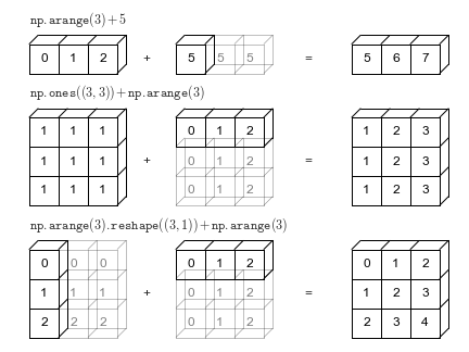\n",
"\n",
"- Additional Sources\n",
" - [Gentle Introduction to Broadcasting](https://machinelearningmastery.com/broadcasting-with-numpy-arrays)\n",
" - [Numpy Broadcasting Docs](https://docs.scipy.org/doc/numpy/user/basics.broadcasting.html)\n",
" - [Introduction to Broadcasting](https://jakevdp.github.io/PythonDataScienceHandbook/02.05-computation-on-arrays-broadcasting.html)"
]
},
{
"cell_type": "markdown",
"id": "e66f201c-e8b5-41fc-9d47-9f71597a0538",
"metadata": {},
"source": [
"**Example 1 - Adding a scalar to an array**\n",
"\n",
"1. Initial shapes: \n",
"Note that `a` is a 1D array and `b` is a scalar and therefore has no shape!\n",
"```\n",
" a.shape = (3,)\n",
" b.shape = ()\n",
"```\n",
"2. Convert to array: \n",
"NumPy first turns the scalar `b` into a 1D array.\n",
"```\n",
" a.shape = (3,)\n",
" b.shape = (1,)\n",
"```\n",
"\n",
"\n",
"3. Apply rule 2: \n",
"NumPy stretches `b` by copying the scalar value of `b` repeatedly until the first dimension of `b` matches the first dimension of `a`. Refer to the above picture where the 5 is copied two more times!\n",
"```\n",
" a.shape = (3,)\n",
" b.shape = (3,)\n",
"```"
]
},
{
"cell_type": "code",
"execution_count": 70,
"id": "58585d80-c0ed-4cf8-a1ba-fdc915aa581c",
"metadata": {},
"outputs": [
{
"data": {
"text/plain": [
"array([5, 6, 7])"
]
},
"execution_count": 70,
"metadata": {},
"output_type": "execute_result"
}
],
"source": [
"a = np.arange(3)\n",
"b = 5\n",
"\n",
"a + 5"
]
},
{
"cell_type": "markdown",
"id": "967e3dc1-feb5-4d0b-ac87-3e7e2aa1e297",
"metadata": {},
"source": [
"**Example 2 - Adding a 1D array to a 2D array (MOST COMMON SCENARIO)**\n",
"1. Beginning shapes:\n",
"```\n",
" A.shape = (3, 3)\n",
" b.shape = (3,)\n",
"```\n",
"\n",
"\n",
"2. Apply rule 1 to `b`: NumPy does so by adding a new dimension to the left of the existing dimensions of `b`.\n",
"\n",
"```\n",
" A.shape = (3, 3)\n",
" b.shape = (1, 3)\n",
"```\n",
"\n",
"\n",
"3. Apply rule 2 to `b`: NumPy stretches `b` by copying `b` repeatedly until the first dimension of `b` matches the first dimension of `A`. Refer to the above picture where `b` is copied two more additional times!\n",
"\n",
"```\n",
" A.shape = (3, 3)\n",
" b.shape = (3, 3)\n",
"```"
]
},
{
"cell_type": "code",
"execution_count": 71,
"id": "cfdddd7e-1ccf-43a4-9870-5727abd2a2f4",
"metadata": {},
"outputs": [
{
"data": {
"text/plain": [
"array([[1., 2., 3.],\n",
" [1., 2., 3.],\n",
" [1., 2., 3.]])"
]
},
"execution_count": 71,
"metadata": {},
"output_type": "execute_result"
}
],
"source": [
"A = np.ones((3, 3))\n",
"b = np.arange(3,)\n",
"\n",
"A + b"
]
},
{
"cell_type": "markdown",
"id": "c2b8c428-0bf9-45c1-9c34-b76c174e9752",
"metadata": {},
"source": [
"**Example 3 - Adding 1D array to a 2D array**\n",
"1. Beginning shapes:\n",
"```\n",
" A.shape = (3, 1)\n",
" b.shape = (3,)\n",
"```\n",
"\n",
"\n",
"2. Apply rule 1 to `b`: NumPy does so by adding a new dimension to the left of the existing dimensions for `b`.\n",
"```\n",
" A.shape = (3, 1)\n",
" b.shape = (1, 3)\n",
"```\n",
"\n",
"\n",
"3. Apply rule 2 to `A` and `b`: \n",
"Notice now NumPy needs to stretch both `A` and `b` so their dimension lengths match! NumPy does this once again by copying the values of `A` and `b` each twice.\n",
"```\n",
" A.shape = (3, 3)\n",
" b.shape = (3, 3)\n",
"```"
]
},
{
"cell_type": "code",
"execution_count": 72,
"id": "5e5ae9da-5848-4ff4-b52b-b923c18ca67e",
"metadata": {},
"outputs": [
{
"data": {
"text/plain": [
"array([[0, 1, 2],\n",
" [1, 2, 3],\n",
" [2, 3, 4]])"
]
},
"execution_count": 72,
"metadata": {},
"output_type": "execute_result"
}
],
"source": [
"A = np.arange(3).reshape((3, 1))\n",
"b = np.arange(3)\n",
"\n",
"A + b"
]
},
{
"cell_type": "markdown",
"id": "35c3469f-d144-4bde-b34e-797ce86c376d",
"metadata": {},
"source": [
"**Example 4 - Broadcasting Error (No corresponding image)**\n",
"1. Beginning shapes:\n",
"```\n",
" A.shape = (3, 2)\n",
" b.shape = (3,)\n",
"```\n",
"2. Apply rule 1 to `b`: \n",
"NumPy does so by adding a new dimension to the left of the existing dimensions for `b`.\n",
"```\n",
" A.shape = (3, 2)\n",
" b.shape = (1, 3)\n",
"```\n",
"\n",
"\n",
"3. Apply rule 2 to `b`:\n",
"NumPy stretches `b` by copying `b` repeatedly until the first dimension of `b` matches the first dimension of `A`. \n",
"```\n",
" A.shape = (3, 2)\n",
" b.shape = (3, 3)\n",
"```\n",
"\n",
"3. Mismatch error is thrown because `A`'s second dimension does not have a length of `1` which means rule 2 can't be applied to it! Meaning, the shapes can not be made to match!\n",
"```\n",
" (3, 2) != (3, 3)\n",
"```"
]
},
{
"cell_type": "code",
"execution_count": 73,
"id": "3f4bd338-d249-4dbb-befe-7f0eabf4811d",
"metadata": {},
"outputs": [
{
"name": "stderr",
"output_type": "stream",
"text": [
"Traceback (most recent call last):\n",
" File \"/tmp/ipykernel_55364/4033666338.py\", line 5, in \n",
" A + b\n",
"ValueError: operands could not be broadcast together with shapes (3,2) (3,) \n"
]
}
],
"source": [
"A = np.ones((3, 2))\n",
"b = np.arange(3)\n",
"\n",
"try:\n",
" A + b\n",
"except ValueError as e:\n",
" traceback.print_exc()"
]
},
{
"cell_type": "markdown",
"id": "c5b387d9-ce10-424d-a29c-03d746e20f55",
"metadata": {},
"source": [
"# Linear Algebra with NumPy\n",
"\n",
"In this section, we will briefly review basic linear algebra concepts and provide code examples using NumPy. Thoroughly go through the below notes as you will need to understand and code ALL concepts covered below."
]
},
{
"cell_type": "markdown",
"id": "206fbdab-7f4f-47f1-9058-173b77d9b181",
"metadata": {
"id": "B7CL-5lqSBf5"
},
"source": [
"## Vectors\n",
"\n",
"Here we will look at **vector** operations and code examples."
]
},
{
"cell_type": "markdown",
"id": "788bafb0-0b9d-42df-80b1-30f7b551fc37",
"metadata": {},
"source": [
"### Defining a 1D Vector\n",
"\n",
"Below, we quickly define a 1D vector and perform check some basic properties of the vector `x`."
]
},
{
"cell_type": "code",
"execution_count": 74,
"id": "3af9e205-1dfd-4d60-893a-f8e4d3df7ff1",
"metadata": {
"colab": {
"base_uri": "https://localhost:8080/"
},
"executionInfo": {
"elapsed": 7,
"status": "ok",
"timestamp": 1720155964064,
"user": {
"displayName": "Minwoo Lee",
"userId": "16199226987142911840"
},
"user_tz": 240
},
"id": "Xssswl5eR8-i",
"outputId": "a23b2e4b-3165-437e-9a33-bca3f800b730"
},
"outputs": [
{
"data": {
"text/plain": [
"array([1, 2, 3])"
]
},
"execution_count": 74,
"metadata": {},
"output_type": "execute_result"
}
],
"source": [
"x = np.array([1, 2, 3])\n",
"x"
]
},
{
"cell_type": "markdown",
"id": "c3f7dac3-e42e-4302-82d6-0b32d19109bb",
"metadata": {},
"source": [
"Here we check the `len()` which returns the length of the 1st dimenision. "
]
},
{
"cell_type": "code",
"execution_count": 75,
"id": "a72886ee-ad84-48ee-a78f-7e8fd6148fcb",
"metadata": {
"colab": {
"base_uri": "https://localhost:8080/"
},
"executionInfo": {
"elapsed": 254,
"status": "ok",
"timestamp": 1720155970966,
"user": {
"displayName": "Minwoo Lee",
"userId": "16199226987142911840"
},
"user_tz": 240
},
"id": "SX9kqUbHSO0I",
"outputId": "6a873dce-9622-4daf-f3ab-dd45770bcfc9"
},
"outputs": [
{
"data": {
"text/plain": [
"3"
]
},
"execution_count": 75,
"metadata": {},
"output_type": "execute_result"
}
],
"source": [
"len(x)"
]
},
{
"cell_type": "markdown",
"id": "58783e60-d855-4752-b9d3-b030c67a8af0",
"metadata": {},
"source": [
"Next we check the shape which returns a tuple containing the length of each dimension. Notice, we have 1 dimension of length 3."
]
},
{
"cell_type": "code",
"execution_count": 76,
"id": "c0459887-b173-4910-89d1-764ed1feb218",
"metadata": {
"colab": {
"base_uri": "https://localhost:8080/"
},
"executionInfo": {
"elapsed": 231,
"status": "ok",
"timestamp": 1720155977506,
"user": {
"displayName": "Minwoo Lee",
"userId": "16199226987142911840"
},
"user_tz": 240
},
"id": "Xs-5PGm1SRvZ",
"outputId": "807d00ad-e080-47e1-9abf-1c817be41bf8"
},
"outputs": [
{
"data": {
"text/plain": [
"(3,)"
]
},
"execution_count": 76,
"metadata": {},
"output_type": "execute_result"
}
],
"source": [
"x.shape"
]
},
{
"cell_type": "markdown",
"id": "7f2cb17d-c4ef-453e-ad88-5252721c474e",
"metadata": {},
"source": [
"Finally, we check both the data type of `x` which is a `np.ndarray` and the data type of an element which is a integer ( see [NumPy data types](https://numpy.org/doc/stable/user/basics.types.html)). "
]
},
{
"cell_type": "code",
"execution_count": 77,
"id": "3ee39e2c-8c10-4458-bace-01dd60af7224",
"metadata": {
"colab": {
"base_uri": "https://localhost:8080/"
},
"executionInfo": {
"elapsed": 185,
"status": "ok",
"timestamp": 1720156010977,
"user": {
"displayName": "Minwoo Lee",
"userId": "16199226987142911840"
},
"user_tz": 240
},
"id": "Ud4gxeg7SX4V",
"outputId": "b6e36db9-52e0-4324-da6d-df92e5ce3d29"
},
"outputs": [
{
"name": "stdout",
"output_type": "stream",
"text": [
"x type: \n",
"x[0] or element type: \n"
]
}
],
"source": [
"print(f\"x type: {type(x)}\")\n",
"print(f\"x[0] or element type: {type(x[0])}\")"
]
},
{
"cell_type": "markdown",
"id": "834cbbee-a570-4505-9a96-1bb1bf5f3897",
"metadata": {},
"source": [
"### Defining 2D Array as a Vector\n",
"\n",
"Recall, we can define a 2D array to represent a vector. Thus, in coding terms the `x_2d` will be a 2d array, but technically it is still a vector since one of the dimensions has a length of 1. This can be a confusing concept to grasp, and a good example of where code and theoretical math differ. "
]
},
{
"cell_type": "markdown",
"id": "3ee40799-c41c-42c2-badf-0d7d735b2f69",
"metadata": {},
"source": [
"Below we define a 2D vector with the shape (1, 3) where the first dimension has length one. Technically, this can be thought of as a row vector as the vector has a single row. A column vector would be the opposite, the shape of (3, 1). "
]
},
{
"cell_type": "code",
"execution_count": 78,
"id": "e3716c55-3abf-4ba7-8d87-ea5e0435751b",
"metadata": {
"colab": {
"base_uri": "https://localhost:8080/"
},
"id": "AEd8jB7YcgtT",
"outputId": "36c31e73-7b57-45c2-8eb3-17900ce131f2"
},
"outputs": [
{
"data": {
"text/plain": [
"array([[1, 2, 3]])"
]
},
"execution_count": 78,
"metadata": {},
"output_type": "execute_result"
}
],
"source": [
"x_2d = np.array([[1, 2, 3]])\n",
"x_2d"
]
},
{
"cell_type": "code",
"execution_count": 79,
"id": "cb719e49-7584-4176-a8fd-ffe48775c79d",
"metadata": {},
"outputs": [
{
"data": {
"text/plain": [
"(1, 3)"
]
},
"execution_count": 79,
"metadata": {},
"output_type": "execute_result"
}
],
"source": [
"x_2d.shape"
]
},
{
"cell_type": "code",
"execution_count": 80,
"id": "70b3f9fa-9083-436b-8472-d07f0bd8942a",
"metadata": {},
"outputs": [
{
"data": {
"text/plain": [
"(numpy.ndarray, numpy.ndarray)"
]
},
"execution_count": 80,
"metadata": {},
"output_type": "execute_result"
}
],
"source": [
"type(x_2d), type(x_2d[0])"
]
},
{
"cell_type": "markdown",
"id": "0dec3d45-06c6-48fe-a604-f12cdf74ae38",
"metadata": {
"colab": {
"base_uri": "https://localhost:8080/"
},
"id": "UHQd92oRcgtV",
"outputId": "2da66795-343c-49a7-86d3-07f96f726245"
},
"source": [
"### Vector Operations\n",
"\n",
"Below are basic vector operations using both 1D and 2D vectors. Before we do, we define another 1D vector `y`."
]
},
{
"cell_type": "code",
"execution_count": 81,
"id": "677aa6f2-ff53-4f3c-945b-79ec320c5456",
"metadata": {},
"outputs": [
{
"name": "stdout",
"output_type": "stream",
"text": [
"y: [2 4 6]\n",
"y.shape: (3,)\n"
]
}
],
"source": [
"y = np.array([2, 4, 6])\n",
"print(f\"y: {y}\")\n",
"print(f\"y.shape: {y.shape}\")"
]
},
{
"cell_type": "markdown",
"id": "60685497-026a-413c-a019-3bfd2d65ef03",
"metadata": {},
"source": [
"#### Addition\n",
"\n",
"Below is code for computing vector addition using the syntax `+`. \n",
"\n",
"First, is matrix-matrix addition, where the vectors are added element-wise. "
]
},
{
"cell_type": "code",
"execution_count": 82,
"id": "6fb21cc6-1439-4193-bb4d-a2947a27c7a4",
"metadata": {},
"outputs": [
{
"data": {
"text/plain": [
"array([3, 6, 9])"
]
},
"execution_count": 82,
"metadata": {},
"output_type": "execute_result"
}
],
"source": [
"x + y"
]
},
{
"cell_type": "markdown",
"id": "692f1cff-a05d-42ff-8a7e-de93f323e086",
"metadata": {},
"source": [
"Next, is matrix-scalar addition, where the scalar is added to each element. "
]
},
{
"cell_type": "code",
"execution_count": 83,
"id": "8107254e-e270-47d7-9959-5dc0813e5c2c",
"metadata": {},
"outputs": [
{
"data": {
"text/plain": [
"array([4, 5, 6])"
]
},
"execution_count": 83,
"metadata": {},
"output_type": "execute_result"
}
],
"source": [
"x + 3"
]
},
{
"cell_type": "markdown",
"id": "8cf0a5cc-58c5-4d46-a1f0-99dc4f617870",
"metadata": {},
"source": [
"#### Subtraction\n",
"\n",
"Below is code for computing vector subtraction using the syntax `-`. \n",
"\n",
"First, is vector-vector subtraction, where the vectors are subtracted element-wise. "
]
},
{
"cell_type": "code",
"execution_count": 84,
"id": "2143266c-0269-4c59-be17-f809632ab026",
"metadata": {},
"outputs": [
{
"data": {
"text/plain": [
"array([-1, -2, -3])"
]
},
"execution_count": 84,
"metadata": {},
"output_type": "execute_result"
}
],
"source": [
"x - y"
]
},
{
"cell_type": "code",
"execution_count": 85,
"id": "d0f2452d-63b5-45b6-874e-ec09e44ed895",
"metadata": {},
"outputs": [
{
"data": {
"text/plain": [
"array([-2, -1, 0])"
]
},
"execution_count": 85,
"metadata": {},
"output_type": "execute_result"
}
],
"source": [
"x - 3"
]
},
{
"cell_type": "markdown",
"id": "c16e93dc-2670-437e-9c29-5061b33a75dc",
"metadata": {},
"source": [
"#### Division\n",
"\n",
"Below is code for computing vector-scalar division using the syntax `/`. Notice the divisor number divides each element."
]
},
{
"cell_type": "code",
"execution_count": 86,
"id": "ebdd38e4-f643-436e-8898-8dee55515bfb",
"metadata": {},
"outputs": [
{
"data": {
"text/plain": [
"array([0.33333333, 0.66666667, 1. ])"
]
},
"execution_count": 86,
"metadata": {},
"output_type": "execute_result"
}
],
"source": [
"x / 3"
]
},
{
"cell_type": "code",
"execution_count": 87,
"id": "12b82136-e91b-4b4f-a2f0-3f932cfa3257",
"metadata": {},
"outputs": [
{
"data": {
"text/plain": [
"array([[0.33333333, 0.66666667, 1. ]])"
]
},
"execution_count": 87,
"metadata": {},
"output_type": "execute_result"
}
],
"source": [
"x_2d / 3"
]
},
{
"cell_type": "markdown",
"id": "ddf5c6d9-352d-4357-b387-d95067eaddd4",
"metadata": {},
"source": [
"#### Power\n",
"\n",
"Below is code for computing raising a vector to a power using the `**` syntax. Notice the power is applied to each element."
]
},
{
"cell_type": "code",
"execution_count": 88,
"id": "0ce28fe9-ecc3-4f3f-abfb-9c7bbbab9ad3",
"metadata": {},
"outputs": [
{
"data": {
"text/plain": [
"array([1, 4, 9])"
]
},
"execution_count": 88,
"metadata": {},
"output_type": "execute_result"
}
],
"source": [
"x ** 2"
]
},
{
"cell_type": "code",
"execution_count": 89,
"id": "674a3f2c-8a94-4c2c-877e-a9f64190cfa9",
"metadata": {},
"outputs": [
{
"data": {
"text/plain": [
"array([[1, 4, 9]])"
]
},
"execution_count": 89,
"metadata": {},
"output_type": "execute_result"
}
],
"source": [
"x_2d ** 2"
]
},
{
"cell_type": "markdown",
"id": "34196c6f-f77f-4b5c-bcc1-b1402ec6b1af",
"metadata": {},
"source": [
"The square-root can then be computed two ways, as seen below."
]
},
{
"cell_type": "code",
"execution_count": 90,
"id": "10c5cc80-9266-42f5-a7aa-9257b999ad7c",
"metadata": {},
"outputs": [
{
"data": {
"text/plain": [
"array([1. , 1.41421356, 1.73205081])"
]
},
"execution_count": 90,
"metadata": {},
"output_type": "execute_result"
}
],
"source": [
"x ** (1/2)"
]
},
{
"cell_type": "code",
"execution_count": 91,
"id": "daa264e0-8d24-4390-9f6f-4ed613cb84b1",
"metadata": {},
"outputs": [
{
"data": {
"text/plain": [
"array([1. , 1.41421356, 1.73205081])"
]
},
"execution_count": 91,
"metadata": {},
"output_type": "execute_result"
}
],
"source": [
"np.sqrt(x)"
]
},
{
"cell_type": "markdown",
"id": "ec151b6b-5e74-4a61-806b-37a70d424120",
"metadata": {},
"source": [
"#### Scalar Multiplication \n",
"Below is code for computing vector-scalar multiplication using the syntax `*`. Notice, each element of `x` is just multiplied by 3."
]
},
{
"cell_type": "code",
"execution_count": 92,
"id": "012fc829-3b98-4652-a2d3-1cc62bb458e4",
"metadata": {},
"outputs": [
{
"data": {
"text/plain": [
"array([3, 6, 9])"
]
},
"execution_count": 92,
"metadata": {},
"output_type": "execute_result"
}
],
"source": [
"x * 3"
]
},
{
"cell_type": "code",
"execution_count": 93,
"id": "c5239b72-b01c-4cf8-bf6d-629ada75b1e5",
"metadata": {},
"outputs": [
{
"data": {
"text/plain": [
"array([3, 6, 9])"
]
},
"execution_count": 93,
"metadata": {},
"output_type": "execute_result"
}
],
"source": [
"3 * x"
]
},
{
"cell_type": "markdown",
"id": "49f50fa0-6118-4e76-8299-891278cc3631",
"metadata": {},
"source": [
"#### Element-wise Multiplication\n",
"\n",
"Below is code for computing element-wise product using the syntax `*`. This is also called the **Hadamard product** (denoted by the $\\odot$ or $*$ operators). Notice, each element in `x` is multiplied by `y`. "
]
},
{
"cell_type": "code",
"execution_count": 94,
"id": "fe2ce72e-f5aa-4976-a053-d4f6333f75ed",
"metadata": {},
"outputs": [
{
"data": {
"text/plain": [
"array([ 2, 8, 18])"
]
},
"execution_count": 94,
"metadata": {},
"output_type": "execute_result"
}
],
"source": [
"x * y"
]
},
{
"cell_type": "markdown",
"id": "bace6273-9cc9-4c8a-b858-e3b61c28bf16",
"metadata": {},
"source": [
"#### Dot Product\n",
"Recall that the dot product is defined as: \n",
"> algebraic operation that takes two equal-length sequences of numbers (usually coordinate vectors), and returns a single number.\n",
"\n",
"To compute the dot product, you can use `np.dot`, `np.matmul` or the overloaded simple notation of `@`. It is worth noting that `@` technically refers to matrix multiplication but also works for computing the dot product in NumPy. The main difference between `@` or `np.matmul` and `np.dot` only really comes into play when dealing with arrays with dimensions greater than 3. For those interested, see this [post](https://stackoverflow.com/questions/34142485/difference-between-numpy-dot-and-python-3-5-matrix-multiplication) on the differences between the functions."
]
},
{
"cell_type": "code",
"execution_count": 95,
"id": "6daba55e-fb3d-48c6-a070-03e62287159c",
"metadata": {},
"outputs": [
{
"data": {
"text/plain": [
"np.int64(28)"
]
},
"execution_count": 95,
"metadata": {},
"output_type": "execute_result"
}
],
"source": [
"x @ y"
]
},
{
"cell_type": "code",
"execution_count": 96,
"id": "38fde9f1-2b42-489d-8593-26f08f619faf",
"metadata": {},
"outputs": [
{
"data": {
"text/plain": [
"np.int64(28)"
]
},
"execution_count": 96,
"metadata": {},
"output_type": "execute_result"
}
],
"source": [
"np.dot(x, y)"
]
},
{
"cell_type": "code",
"execution_count": 97,
"id": "262c099d-37aa-464e-9378-72d59ba165e0",
"metadata": {},
"outputs": [
{
"data": {
"text/plain": [
"np.int64(28)"
]
},
"execution_count": 97,
"metadata": {},
"output_type": "execute_result"
}
],
"source": [
"np.matmul(x, y)"
]
},
{
"cell_type": "code",
"execution_count": 98,
"id": "c3d609a3-f551-4c90-8f1f-2cadb5ad3c7f",
"metadata": {},
"outputs": [
{
"data": {
"text/plain": [
"array([28])"
]
},
"execution_count": 98,
"metadata": {},
"output_type": "execute_result"
}
],
"source": [
"x_2d @ y"
]
},
{
"cell_type": "code",
"execution_count": 99,
"id": "d803ba79-fc44-4951-9e65-dc289cd3b7eb",
"metadata": {},
"outputs": [
{
"data": {
"text/plain": [
"array([28])"
]
},
"execution_count": 99,
"metadata": {},
"output_type": "execute_result"
}
],
"source": [
"np.dot(x_2d, y)"
]
},
{
"cell_type": "markdown",
"id": "6b12eb67-6295-4618-86d7-08b99cc55ea3",
"metadata": {},
"source": [
"Below is an example of reshaping an 2D vector so that we do not get a matmul error!"
]
},
{
"cell_type": "code",
"execution_count": 100,
"id": "eacf555f-81ff-4baf-9951-44175ac841e5",
"metadata": {},
"outputs": [
{
"data": {
"text/plain": [
"array([28])"
]
},
"execution_count": 100,
"metadata": {},
"output_type": "execute_result"
}
],
"source": [
"y @ x_2d.reshape(-1, 1)"
]
},
{
"cell_type": "markdown",
"id": "6cfcdbd0-d8cf-471a-a388-10217b2e7997",
"metadata": {
"id": "NiEofCzYZBrQ"
},
"source": [
"#### Transposition\n",
"\n",
"Below we display how to take the transpose of a vector."
]
},
{
"cell_type": "markdown",
"id": "f82e06b5-7d18-47f0-923d-c220afb02f99",
"metadata": {},
"source": [
"Now let's transpose a vector using the `.T` syntax. Notice, transposing has no effect on a 1D vector. "
]
},
{
"cell_type": "code",
"execution_count": 101,
"id": "6160658e-c15f-493b-b243-3f46f49c7da1",
"metadata": {},
"outputs": [
{
"data": {
"text/plain": [
"array([1, 2, 3])"
]
},
"execution_count": 101,
"metadata": {},
"output_type": "execute_result"
}
],
"source": [
"x_t = x.T\n",
"x_t"
]
},
{
"cell_type": "code",
"execution_count": 102,
"id": "14b2c782-3311-4db4-b32e-332e34644d7e",
"metadata": {},
"outputs": [
{
"data": {
"text/plain": [
"(3,)"
]
},
"execution_count": 102,
"metadata": {},
"output_type": "execute_result"
}
],
"source": [
"x_t.shape"
]
},
{
"cell_type": "markdown",
"id": "2fbdf248-3bde-48d1-8ce9-3832dd79c7cb",
"metadata": {},
"source": [
"Yet, if we transpose a 2D vector, the dimension of length 1 changes and now we have a column vector."
]
},
{
"cell_type": "code",
"execution_count": 103,
"id": "f5f905ee-3fe3-4576-8a2c-c665d643934e",
"metadata": {
"colab": {
"base_uri": "https://localhost:8080/"
},
"id": "hxGFNDx6V95l",
"outputId": "21af3de1-9621-41a3-9839-64f7ab7d94a2"
},
"outputs": [
{
"data": {
"text/plain": [
"array([[1],\n",
" [2],\n",
" [3]])"
]
},
"execution_count": 103,
"metadata": {},
"output_type": "execute_result"
}
],
"source": [
"x_2d_t = x_2d.T\n",
"x_2d_t"
]
},
{
"cell_type": "code",
"execution_count": 104,
"id": "36ccc514-c92d-41a4-a8a9-af28ccbf5715",
"metadata": {
"colab": {
"base_uri": "https://localhost:8080/"
},
"id": "_f8E9ExDWw4p",
"outputId": "8c1c6d11-250d-4a59-d4a1-82e74ae618ee"
},
"outputs": [
{
"data": {
"text/plain": [
"(3, 1)"
]
},
"execution_count": 104,
"metadata": {},
"output_type": "execute_result"
}
],
"source": [
"x_2d_t.shape"
]
},
{
"cell_type": "markdown",
"id": "6557df88-a675-48e7-8408-871b7ded9994",
"metadata": {},
"source": [
"We can recover the original 2D row vector by simply transposing again. "
]
},
{
"cell_type": "code",
"execution_count": 105,
"id": "9abe4547-11aa-41d6-8757-52fa13a4a6b2",
"metadata": {},
"outputs": [
{
"data": {
"text/plain": [
"array([[1, 2, 3]])"
]
},
"execution_count": 105,
"metadata": {},
"output_type": "execute_result"
}
],
"source": [
"x_2d_t_t = x_2d_t.T\n",
"x_2d_t_t"
]
},
{
"cell_type": "code",
"execution_count": 106,
"id": "4e147575-2421-4764-aef4-37adb3568797",
"metadata": {},
"outputs": [
{
"data": {
"text/plain": [
"(1, 3)"
]
},
"execution_count": 106,
"metadata": {},
"output_type": "execute_result"
}
],
"source": [
"x_2d_t_t.shape"
]
},
{
"cell_type": "markdown",
"id": "85d8bc56-ea0b-4f76-a6f4-3da017ee8e4d",
"metadata": {
"id": "Ta9IQK5AO97s"
},
"source": [
"## Matrices\n",
"\n",
"Here we will look at **matrix** operations and code examples."
]
},
{
"cell_type": "markdown",
"id": "294156fb-e6ef-4e5d-b2de-9ea68b13e6fe",
"metadata": {},
"source": [
"### Defining a 2D Matrix\n",
"\n",
"Below, we quickly define a 2D matrix and perform check some basic properties of the matrix `X`. \n",
"\n",
"To define `X` we use `np.arange` to create a 1D vector of shape (6), then we use `.reshape` to reshape it into a (3, 2) matrix."
]
},
{
"cell_type": "code",
"execution_count": 107,
"id": "d3943b96-96b0-46e2-8548-f63393a32e89",
"metadata": {
"id": "IGBRfMVjO97s",
"outputId": "671a858f-36de-43f9-c40c-cdd43ad4087a"
},
"outputs": [
{
"data": {
"text/plain": [
"array([[0, 1],\n",
" [2, 3],\n",
" [4, 5]])"
]
},
"execution_count": 107,
"metadata": {},
"output_type": "execute_result"
}
],
"source": [
"X = np.arange(6).reshape((3,2))\n",
"X"
]
},
{
"cell_type": "code",
"execution_count": 108,
"id": "483ed86f-4558-46d8-a2dc-e513c89dc3b7",
"metadata": {},
"outputs": [
{
"data": {
"text/plain": [
"(3, 2)"
]
},
"execution_count": 108,
"metadata": {},
"output_type": "execute_result"
}
],
"source": [
"X.shape"
]
},
{
"cell_type": "markdown",
"id": "c9420306-143b-4417-97fc-9b29344eb1ce",
"metadata": {},
"source": [
"Now, notice that we have to index both dimensions (row and column) to get a specific element data type. If we just index the row or column we get a vector which is another `np.ndarray` type."
]
},
{
"cell_type": "code",
"execution_count": 109,
"id": "837d495e-3238-462f-8103-ef054f605793",
"metadata": {},
"outputs": [
{
"name": "stdout",
"output_type": "stream",
"text": [
"X type: \n",
"X[0] or row type: \n",
"X[0, 0] or element type: \n"
]
}
],
"source": [
"print(f\"X type: {type(X)}\")\n",
"print(f\"X[0] or row type: {type(X[0])}\")\n",
"print(f\"X[0, 0] or element type: {type(X[0, 0])}\")"
]
},
{
"cell_type": "markdown",
"id": "92d29190-7411-43bb-ba79-ec9443443ca9",
"metadata": {},
"source": [
"### Matrix Operations\n",
"\n",
"Below are basic matrix for 2D matrices. Before we do, we define another 2D matrix `A`."
]
},
{
"cell_type": "code",
"execution_count": 110,
"id": "e8399b57-fcc2-4a65-a0f4-b35e04052e44",
"metadata": {},
"outputs": [
{
"data": {
"text/plain": [
"array([[ 5, 6],\n",
" [ 7, 8],\n",
" [ 9, 10]])"
]
},
"execution_count": 110,
"metadata": {},
"output_type": "execute_result"
}
],
"source": [
"A = np.arange(5,11).reshape((3,2))\n",
"A"
]
},
{
"cell_type": "code",
"execution_count": 111,
"id": "a783f6e8-9bb5-4172-af26-e26d3d5ef9e5",
"metadata": {},
"outputs": [
{
"data": {
"text/plain": [
"(3, 2)"
]
},
"execution_count": 111,
"metadata": {},
"output_type": "execute_result"
}
],
"source": [
"A.shape"
]
},
{
"cell_type": "markdown",
"id": "05de7cc0-e0d7-4536-a4f5-25b051864f27",
"metadata": {},
"source": [
"#### Addition\n",
"\n",
"Below is code for computing matrix addition using the syntax `+`. \n",
"\n",
"First, is matrix-matrix addition, where the matrices are added element-wise. "
]
},
{
"cell_type": "code",
"execution_count": 112,
"id": "d41ed0d0-41c5-46c8-b9a2-b1592b0c0a72",
"metadata": {
"id": "K6Lv6Kc_O97s",
"outputId": "a1c797af-a237-4de5-f03a-0dafa5544cd3"
},
"outputs": [
{
"data": {
"text/plain": [
"array([[ 5, 7],\n",
" [ 9, 11],\n",
" [13, 15]])"
]
},
"execution_count": 112,
"metadata": {},
"output_type": "execute_result"
}
],
"source": [
"X + A"
]
},
{
"cell_type": "markdown",
"id": "8674a28e-004c-4145-adb6-5f476f37e2b2",
"metadata": {},
"source": [
"Next, is matrix-scalar addition, where the scalar is added to each element. "
]
},
{
"cell_type": "code",
"execution_count": 113,
"id": "f8f1958c-4e7c-4239-8acc-9f83b4118c4c",
"metadata": {},
"outputs": [
{
"data": {
"text/plain": [
"array([[ 8, 9],\n",
" [10, 11],\n",
" [12, 13]])"
]
},
"execution_count": 113,
"metadata": {},
"output_type": "execute_result"
}
],
"source": [
"A + 3"
]
},
{
"cell_type": "markdown",
"id": "36b8d75d-812d-4c5f-9d42-7133729f7e09",
"metadata": {},
"source": [
"#### Subtraction\n",
"\n",
"Below is code for computing matrix subtraction using the syntax `-`. \n",
"\n",
"First, is vector-vector subtraction, where the vectors are subtracted element-wise. "
]
},
{
"cell_type": "code",
"execution_count": 114,
"id": "946c2474-0aa0-4fe2-a291-c818d4de124d",
"metadata": {
"id": "gdwIhiiYO97s",
"outputId": "51e7c78a-e968-49eb-cc7c-2d5e010dcdc1"
},
"outputs": [
{
"data": {
"text/plain": [
"array([[-5, -5],\n",
" [-5, -5],\n",
" [-5, -5]])"
]
},
"execution_count": 114,
"metadata": {},
"output_type": "execute_result"
}
],
"source": [
"X - A"
]
},
{
"cell_type": "markdown",
"id": "d2821a7a-ec00-4d18-b045-f81c4f7799d0",
"metadata": {},
"source": [
"Next, is matrix-scalar subtraction, where the scalar is subtracted to each element. "
]
},
{
"cell_type": "code",
"execution_count": 115,
"id": "c55782c8-7354-436c-b726-6bca63bcd88c",
"metadata": {},
"outputs": [
{
"data": {
"text/plain": [
"array([[-3, -2],\n",
" [-1, 0],\n",
" [ 1, 2]])"
]
},
"execution_count": 115,
"metadata": {},
"output_type": "execute_result"
}
],
"source": [
"X - 3"
]
},
{
"cell_type": "markdown",
"id": "68e050cb-6276-44cd-9c1b-73130369fe9e",
"metadata": {},
"source": [
"#### Division\n",
"\n",
"Below is code for computing matrix-scalar division using the syntax `/`. Notice the divisor number divides each element."
]
},
{
"cell_type": "code",
"execution_count": 116,
"id": "964c0e66-65e6-43ff-a1d5-4e008d08d403",
"metadata": {},
"outputs": [
{
"data": {
"text/plain": [
"array([[0. , 0.33333333],\n",
" [0.66666667, 1. ],\n",
" [1.33333333, 1.66666667]])"
]
},
"execution_count": 116,
"metadata": {},
"output_type": "execute_result"
}
],
"source": [
"X / 3"
]
},
{
"cell_type": "markdown",
"id": "6426045f-b6da-4f07-8b44-4c73e382154f",
"metadata": {},
"source": [
"#### Power\n",
"\n",
"Below is code for computing raising a matrix to a power using the `**` syntax. Notice the power is applied to each element."
]
},
{
"cell_type": "code",
"execution_count": 117,
"id": "629d8c65-bb39-449a-a5dd-874d687da94a",
"metadata": {},
"outputs": [
{
"data": {
"text/plain": [
"array([[ 0, 1],\n",
" [ 4, 9],\n",
" [16, 25]])"
]
},
"execution_count": 117,
"metadata": {},
"output_type": "execute_result"
}
],
"source": [
"X ** 2"
]
},
{
"cell_type": "markdown",
"id": "8fd8eea5-66ba-46de-867c-341ab9e6cf2f",
"metadata": {},
"source": [
"The square-root can then be computed two ways, as seen below."
]
},
{
"cell_type": "code",
"execution_count": 118,
"id": "d06808d0-ae87-4f79-9543-e0c832a5f301",
"metadata": {},
"outputs": [
{
"data": {
"text/plain": [
"array([[0. , 1. ],\n",
" [1.41421356, 1.73205081],\n",
" [2. , 2.23606798]])"
]
},
"execution_count": 118,
"metadata": {},
"output_type": "execute_result"
}
],
"source": [
"X ** (1/2)"
]
},
{
"cell_type": "code",
"execution_count": 119,
"id": "7793c4df-bc7c-46bf-a85e-629cc57ccef8",
"metadata": {},
"outputs": [
{
"data": {
"text/plain": [
"array([[0. , 1. ],\n",
" [1.41421356, 1.73205081],\n",
" [2. , 2.23606798]])"
]
},
"execution_count": 119,
"metadata": {},
"output_type": "execute_result"
}
],
"source": [
"np.sqrt(X)"
]
},
{
"cell_type": "markdown",
"id": "4f716a01-4d0c-43c2-8415-0d260252596e",
"metadata": {},
"source": [
"#### Scalar Multiplication \n",
"Below is code for computing matrix-scalar multiplication using the syntax `*`. Notice, each element of `X` is just multiplied by 3."
]
},
{
"cell_type": "code",
"execution_count": 120,
"id": "b914df16-c870-4660-b228-ced93cff8b43",
"metadata": {
"id": "FljUIHQvO97s",
"outputId": "09948f15-51d7-4100-c107-f563f58958a2"
},
"outputs": [
{
"data": {
"text/plain": [
"array([[ 0, 3],\n",
" [ 6, 9],\n",
" [12, 15]])"
]
},
"execution_count": 120,
"metadata": {},
"output_type": "execute_result"
}
],
"source": [
"X * 3"
]
},
{
"cell_type": "code",
"execution_count": 121,
"id": "f38e324a-bb59-4298-9720-225677e7cc21",
"metadata": {},
"outputs": [
{
"data": {
"text/plain": [
"array([[ 0, 3],\n",
" [ 6, 9],\n",
" [12, 15]])"
]
},
"execution_count": 121,
"metadata": {},
"output_type": "execute_result"
}
],
"source": [
"3 * X"
]
},
{
"cell_type": "markdown",
"id": "2055e281-7fc0-4072-a7a0-cbdd63423607",
"metadata": {},
"source": [
"#### Element-wise Multiplication\n",
"\n",
"Below is code for computing element-wise product using the syntax `*`. This is also called the **Hadamard product** (denoted by the $\\odot$ or $*$ operators). Notice, each element in `X` is multiplied by `A`. "
]
},
{
"cell_type": "code",
"execution_count": 122,
"id": "c60391cd-6d34-4912-9910-da6fcdb8d8e2",
"metadata": {},
"outputs": [
{
"data": {
"text/plain": [
"array([[ 0, 6],\n",
" [14, 24],\n",
" [36, 50]])"
]
},
"execution_count": 122,
"metadata": {},
"output_type": "execute_result"
}
],
"source": [
"X * A"
]
},
{
"cell_type": "markdown",
"id": "5f345c49-862c-43c5-a280-7da9ff47130a",
"metadata": {},
"source": [
"#### Matrix Multiplication \n",
"\n",
"Recall the definition of matrix multiplication as follows:\n",
"\n",
"> matrix multiplication is a binary operation that produces a matrix from two matrices. For matrix multiplication, the number of columns in the first matrix must be equal to the number of rows in the second matrix. The resulting matrix, known as the matrix product, has the number of rows of the first and the number of columns of the second matrix.\n",
"\n",
"\n",
"The equivalent of the dot product for matrices is referred to as matrix multiplication. Often times people will overload the term dot product though to also refer to matrix multiplication, which is technically incorrect. \n",
"\n"
]
},
{
"cell_type": "markdown",
"id": "cb37425f-35e7-455d-b2ac-ce067a924bfd",
"metadata": {},
"source": [
"To compute the matrix product, you can use `np.dot`, `np.matmul` or the overloaded simple notation of `@`. It is worth noting that `@` technically refers to matrix multiplication but also works for computing the dot product in NumPy. The main difference between `@` or `np.matmul` and `np.dot` only really comes into play when dealing with arrays with dimensions greater than 3. For those interested, see this [post](https://stackoverflow.com/questions/34142485/difference-between-numpy-dot-and-python-3-5-matrix-multiplication) on the differences between the functions."
]
},
{
"cell_type": "code",
"execution_count": 123,
"id": "98fc3446-d11b-4d3c-8107-99e27d16ed58",
"metadata": {},
"outputs": [
{
"data": {
"text/plain": [
"array([[1., 1., 1.],\n",
" [1., 1., 1.]])"
]
},
"execution_count": 123,
"metadata": {},
"output_type": "execute_result"
}
],
"source": [
"B = np.ones((2,3))\n",
"B"
]
},
{
"cell_type": "code",
"execution_count": 124,
"id": "a098ed12-3e18-45b7-957c-4249e1f83b0d",
"metadata": {},
"outputs": [
{
"data": {
"text/plain": [
"array([[1., 1., 1.],\n",
" [5., 5., 5.],\n",
" [9., 9., 9.]])"
]
},
"execution_count": 124,
"metadata": {},
"output_type": "execute_result"
}
],
"source": [
"np.dot(X, B)"
]
},
{
"cell_type": "code",
"execution_count": 125,
"id": "3eef72a6-34c3-438d-9439-49ea6e5b6d4f",
"metadata": {},
"outputs": [
{
"data": {
"text/plain": [
"array([[1., 1., 1.],\n",
" [5., 5., 5.],\n",
" [9., 9., 9.]])"
]
},
"execution_count": 125,
"metadata": {},
"output_type": "execute_result"
}
],
"source": [
"np.matmul(X, B)"
]
},
{
"cell_type": "code",
"execution_count": 126,
"id": "2fe47b67-ba08-4c7d-a3e8-9271326467ed",
"metadata": {},
"outputs": [
{
"data": {
"text/plain": [
"array([[1., 1., 1.],\n",
" [5., 5., 5.],\n",
" [9., 9., 9.]])"
]
},
"execution_count": 126,
"metadata": {},
"output_type": "execute_result"
}
],
"source": [
"X @ B"
]
},
{
"cell_type": "markdown",
"id": "a7a2d904-ec0f-45e3-825c-d24832f9e5e9",
"metadata": {},
"source": [
"If we want to compute the matrix product between `X` and `A` we need to reshape or transpose one of the matrices."
]
},
{
"cell_type": "code",
"execution_count": 127,
"id": "696cdc24-6909-4aa2-9463-0d958d318b80",
"metadata": {},
"outputs": [
{
"data": {
"text/plain": [
"array([[0, 1],\n",
" [2, 3],\n",
" [4, 5]])"
]
},
"execution_count": 127,
"metadata": {},
"output_type": "execute_result"
}
],
"source": [
"X"
]
},
{
"cell_type": "code",
"execution_count": 128,
"id": "e7d77a2c-c2d3-49d6-9cc7-dbd39a852575",
"metadata": {},
"outputs": [
{
"data": {
"text/plain": [
"array([[ 5, 7, 9],\n",
" [ 6, 8, 10]])"
]
},
"execution_count": 128,
"metadata": {},
"output_type": "execute_result"
}
],
"source": [
"A.T"
]
},
{
"cell_type": "code",
"execution_count": 129,
"id": "173aafb0-7be7-4d35-ac82-f72a8aede6e6",
"metadata": {},
"outputs": [
{
"data": {
"text/plain": [
"array([[ 6, 8, 10],\n",
" [28, 38, 48],\n",
" [50, 68, 86]])"
]
},
"execution_count": 129,
"metadata": {},
"output_type": "execute_result"
}
],
"source": [
"X @ A.T"
]
},
{
"cell_type": "markdown",
"id": "6dac441e-dd81-496f-9daf-69636470bd16",
"metadata": {
"id": "pC1rWTlVj3Vg"
},
"source": [
"#### Transposition\n",
"\n",
"Now let's transpose a matrix using the `.T` syntax"
]
},
{
"cell_type": "code",
"execution_count": 130,
"id": "15a27798-edb4-475d-bb7d-f2f29d46e14c",
"metadata": {
"colab": {
"base_uri": "https://localhost:8080/"
},
"id": "e7siMBsRj3Vi",
"outputId": "c08f5fb4-b4bf-433b-bb05-cdf9039d3732"
},
"outputs": [
{
"data": {
"text/plain": [
"array([[0, 2, 4],\n",
" [1, 3, 5]])"
]
},
"execution_count": 130,
"metadata": {},
"output_type": "execute_result"
}
],
"source": [
"X_t = X.T\n",
"X_t"
]
},
{
"cell_type": "code",
"execution_count": 131,
"id": "2a5d00f8-a4fe-4a52-8ad2-b89cfa016a34",
"metadata": {},
"outputs": [
{
"data": {
"text/plain": [
"(2, 3)"
]
},
"execution_count": 131,
"metadata": {},
"output_type": "execute_result"
}
],
"source": [
"X_t.shape"
]
},
{
"cell_type": "markdown",
"id": "5336676c-8a92-46fa-a094-66cdd796e468",
"metadata": {},
"source": [
"Once again, we can take the transpose of the transpose `X_t` to get back the original shape. "
]
},
{
"cell_type": "code",
"execution_count": 132,
"id": "ab56d821-b3a2-4194-81f5-6b7a7949578a",
"metadata": {},
"outputs": [
{
"data": {
"text/plain": [
"(3, 2)"
]
},
"execution_count": 132,
"metadata": {},
"output_type": "execute_result"
}
],
"source": [
"X_t.T.shape"
]
},
{
"cell_type": "markdown",
"id": "bdc9ee1b-d8e7-4032-991b-444dea91ccfd",
"metadata": {},
"source": [
"#### Trace\n",
"\n",
"To compute the trace, simply pass a matrix to the `np.trace()` function."
]
},
{
"cell_type": "code",
"execution_count": 133,
"id": "c3561eb5-f800-48dc-9821-6c7280640069",
"metadata": {},
"outputs": [
{
"data": {
"text/plain": [
"array([[1, 2, 3],\n",
" [4, 5, 6],\n",
" [7, 8, 9]])"
]
},
"execution_count": 133,
"metadata": {},
"output_type": "execute_result"
}
],
"source": [
"C = np.arange(1,10).reshape(3,3)\n",
"C"
]
},
{
"cell_type": "code",
"execution_count": 134,
"id": "9fa8cf4d-d34e-45f1-9da1-09257e95f22f",
"metadata": {
"id": "X0hAfnPQO97w",
"outputId": "498dac7e-b1bc-4b63-e310-c098dd0fb8ee"
},
"outputs": [
{
"data": {
"text/plain": [
"np.int64(15)"
]
},
"execution_count": 134,
"metadata": {},
"output_type": "execute_result"
}
],
"source": [
"np.trace(C)"
]
},
{
"cell_type": "markdown",
"id": "cc2167e6-1d63-446a-aa6b-779f98acc1e3",
"metadata": {},
"source": [
"If we do not pass a square matrix, it will still only add those values along the diagonal. "
]
},
{
"cell_type": "code",
"execution_count": 135,
"id": "02c8963f-e4dc-4669-8467-59bd6b4bc65c",
"metadata": {},
"outputs": [
{
"data": {
"text/plain": [
"array([[0, 1],\n",
" [2, 3],\n",
" [4, 5]])"
]
},
"execution_count": 135,
"metadata": {},
"output_type": "execute_result"
}
],
"source": [
"X"
]
},
{
"cell_type": "code",
"execution_count": 136,
"id": "03d4c32f-5970-46b2-9203-eb2f4ea77741",
"metadata": {},
"outputs": [
{
"data": {
"text/plain": [
"np.int64(3)"
]
},
"execution_count": 136,
"metadata": {},
"output_type": "execute_result"
}
],
"source": [
"np.trace(X)"
]
},
{
"cell_type": "markdown",
"id": "c8971f7d-6eec-4dad-8288-53ccad516d0a",
"metadata": {},
"source": [
"#### Rank\n",
"\n",
"\n",
"To compute the rank, simply pass a matrix to the `np.linalg.matrix_rank()` function."
]
},
{
"cell_type": "code",
"execution_count": 137,
"id": "c0f714ea-2b57-44fe-a2c1-6d00af49ea0b",
"metadata": {
"id": "F2jnkoK5O97x",
"outputId": "377e7f18-9593-47b5-9800-0cfb649ac649"
},
"outputs": [
{
"data": {
"text/plain": [
"np.int64(2)"
]
},
"execution_count": 137,
"metadata": {},
"output_type": "execute_result"
}
],
"source": [
"np.linalg.matrix_rank(X)"
]
},
{
"cell_type": "markdown",
"id": "73b8c48d-ce06-4445-8403-c6dbe5b5b400",
"metadata": {
"id": "eCFqu8LWj3WJ"
},
"source": [
"#### Inverse\n",
"\n",
"Likewise, to compute the inverse of a matrix, there are two functions to use: `np.inv` and `np.pinv`. `np.inv` is used to compute the matrix inverse normally, while `np.pinv` using pseudo-inverse to compute inverse for matrices that might not have an inverse. "
]
},
{
"cell_type": "code",
"execution_count": 138,
"id": "4ecfd390-6911-48b3-86af-4040e80f0b0c",
"metadata": {
"colab": {
"base_uri": "https://localhost:8080/"
},
"id": "Hhr16-XVj3WK",
"outputId": "bcd77f90-b2ea-4a56-f17a-e9d5b8f188ab"
},
"outputs": [
{
"data": {
"text/plain": [
"array([[ 4, 2],\n",
" [-5, -3]])"
]
},
"execution_count": 138,
"metadata": {},
"output_type": "execute_result"
}
],
"source": [
"D = np.array([[4, 2], [-5, -3]])\n",
"D"
]
},
{
"cell_type": "code",
"execution_count": 139,
"id": "e45d8f42-3833-46ac-a2c7-05c7c563fd9a",
"metadata": {
"colab": {
"base_uri": "https://localhost:8080/"
},
"id": "FIGmFK9oj3WM",
"outputId": "e1f07c91-957f-4753-b33f-85facd606219"
},
"outputs": [
{
"data": {
"text/plain": [
"array([[ 1.5, 1. ],\n",
" [-2.5, -2. ]])"
]
},
"execution_count": 139,
"metadata": {},
"output_type": "execute_result"
}
],
"source": [
"Dinv = np.linalg.inv(D)\n",
"Dinv"
]
},
{
"cell_type": "code",
"execution_count": 140,
"id": "e48076a0-06b0-41a9-bb09-a348fdd21f99",
"metadata": {
"id": "_WxxXUcIO97z",
"outputId": "4165ba37-43a9-495f-bd81-e7a3fa88954c"
},
"outputs": [
{
"data": {
"text/plain": [
"array([[ 4., 2.],\n",
" [-5., -3.]])"
]
},
"execution_count": 140,
"metadata": {},
"output_type": "execute_result"
}
],
"source": [
"np.linalg.inv(Dinv)"
]
}
],
"metadata": {
"kernelspec": {
"display_name": "Python 3 (ipykernel)",
"language": "python",
"name": "python3"
},
"language_info": {
"codemirror_mode": {
"name": "ipython",
"version": 3
},
"file_extension": ".py",
"mimetype": "text/x-python",
"name": "python",
"nbconvert_exporter": "python",
"pygments_lexer": "ipython3",
"version": "3.10.14"
}
},
"nbformat": 4,
"nbformat_minor": 5
}
\n",
"\n",
"- Additional Sources\n",
" - [How to Set Axis for Rows and Columns in NumPy](https://machinelearningmastery.com/numpy-axis-for-rows-and-columns/)\n",
" - [NumPy Axes explained](https://www.sharpsightlabs.com/blog/numpy-axes-explained/)"
]
},
{
"cell_type": "markdown",
"id": "a9ce8a82-77c3-431d-a76d-eb1b437caf66",
"metadata": {},
"source": [
"Let's create a simply array with a shape of (3, 4). Notice, we use NumPy's `arange` function ([docs](https://numpy.org/doc/stable/reference/generated/numpy.arange.html)) to quickly generate 3 1D arrays and `vstack` ([docs](https://numpy.org/doc/stable/reference/generated/numpy.vstack.html)) function to stack said arrays into a (3, 4) array."
]
},
{
"cell_type": "code",
"execution_count": 31,
"id": "59d8eec8-ebdc-4c4f-99ed-8cf2da6da40d",
"metadata": {},
"outputs": [
{
"name": "stdout",
"output_type": "stream",
"text": [
"axis_array output: \n",
" [[1 2 3 4]\n",
" [1 2 3 4]\n",
" [1 2 3 4]]\n",
"axis_array shap|e: (3, 4)\n"
]
}
],
"source": [
"axis_array = np.vstack([np.arange(1,5), np.arange(1,5), np.arange(1,5)])\n",
"\n",
"print(f\"axis_array output: \\n {axis_array}\")\n",
"print(f\"axis_array shap|e: {axis_array.shape}\")"
]
},
{
"cell_type": "markdown",
"id": "771f3d95-529d-4512-b35a-15b765961823",
"metadata": {},
"source": [
"Alternatively, we could have used NumPy's `stack` function ([docs](https://numpy.org/doc/stable/reference/generated/numpy.stack.html)) and specified `axis=0` to indicate we have to vertically stack each array on top of one another."
]
},
{
"cell_type": "code",
"execution_count": 32,
"id": "03ad7c9b-8f11-4bf8-8d98-667824603959",
"metadata": {},
"outputs": [
{
"name": "stdout",
"output_type": "stream",
"text": [
"axis_array output: \n",
" [[1 2 3 4]\n",
" [1 2 3 4]\n",
" [1 2 3 4]]\n",
"axis_array shape: (3, 4)\n"
]
}
],
"source": [
"axis_array = np.stack([np.arange(1,5), np.arange(1,5), np.arange(1,5)], axis=0)\n",
"\n",
"print(f\"axis_array output: \\n {axis_array}\")\n",
"print(f\"axis_array shape: {axis_array.shape}\")"
]
},
{
"cell_type": "markdown",
"id": "4ee30bbe-1191-495e-afcf-93c465a9fd7b",
"metadata": {},
"source": [
"Here we take the sum with no axis parameter given (in other words, `axis=None` by default). Thus, the sum of the entire array is computed."
]
},
{
"cell_type": "code",
"execution_count": 33,
"id": "eff5ac5b-2f3a-4e97-86e7-ee5d6f2586d7",
"metadata": {},
"outputs": [
{
"data": {
"text/plain": [
"np.int64(30)"
]
},
"execution_count": 33,
"metadata": {},
"output_type": "execute_result"
}
],
"source": [
"np.sum(axis_array)"
]
},
{
"cell_type": "markdown",
"id": "238752ec-4d60-447f-b8cc-c6296fb0ea68",
"metadata": {},
"source": [
"Likewise, we can apply the same idea to the `max` function where the max of the entire array is taken."
]
},
{
"cell_type": "code",
"execution_count": 34,
"id": "5f93eefa-2b60-4188-9331-de51cef2d45b",
"metadata": {},
"outputs": [
{
"data": {
"text/plain": [
"np.int64(4)"
]
},
"execution_count": 34,
"metadata": {},
"output_type": "execute_result"
}
],
"source": [
"np.max(axis_array)"
]
},
{
"cell_type": "markdown",
"id": "63ce0555-205a-4c29-847e-7b7dc1acc86b",
"metadata": {},
"source": [
"Here we take the sum and max for each column by passing `axis=0` which means the 1st dimension (the row dimension) is collapsed. Meaning, we now want to take the sum/max across columns! \n",
"\n",
"Alternatively, think about the axis visually. Recall, `axis=0` points down vertically (see above picture). This means the operation is applied for each column."
]
},
{
"cell_type": "code",
"execution_count": 35,
"id": "44eec937-e66d-4bfa-a970-c6b393141d21",
"metadata": {},
"outputs": [
{
"data": {
"text/plain": [
"array([ 3, 6, 9, 12])"
]
},
"execution_count": 35,
"metadata": {},
"output_type": "execute_result"
}
],
"source": [
"# Column-wise: 1 number for each column\n",
"np.sum(axis_array, axis=0)"
]
},
{
"cell_type": "code",
"execution_count": 36,
"id": "b9faa5d7-9bed-4cab-9973-e926e944061a",
"metadata": {},
"outputs": [
{
"data": {
"text/plain": [
"array([1, 2, 3, 4])"
]
},
"execution_count": 36,
"metadata": {},
"output_type": "execute_result"
}
],
"source": [
"# Another example but now using max\n",
"np.max(axis_array, axis=0)"
]
},
{
"cell_type": "markdown",
"id": "9282a978-9d67-4e6b-be2a-a56b8a7d1c65",
"metadata": {},
"source": [
"Here we take the sum and max row-wise (for each row) by passing `axis=1` which means the 2nd dimension (the column dimension) is collapsed. Meaning, we now want to take the sum/max across rows!\n",
"\n",
"Alternatively, think about the axis visually. Recall, `axis=1` points across the array horizontally (see above picture). This means the operation is applied for each row."
]
},
{
"cell_type": "code",
"execution_count": 37,
"id": "aa50750d-8bc9-473a-980f-7822ff1c313e",
"metadata": {},
"outputs": [
{
"data": {
"text/plain": [
"array([10, 10, 10])"
]
},
"execution_count": 37,
"metadata": {},
"output_type": "execute_result"
}
],
"source": [
"# Row-wise: 1 number for each row\n",
"np.sum(axis_array, axis=1)"
]
},
{
"cell_type": "code",
"execution_count": 38,
"id": "381aa9db-6c1a-461f-94ca-bc5e58841489",
"metadata": {},
"outputs": [
{
"data": {
"text/plain": [
"array([4, 4, 4])"
]
},
"execution_count": 38,
"metadata": {},
"output_type": "execute_result"
}
],
"source": [
"# Another example but now using max\n",
"np.max(axis_array, axis=1)"
]
},
{
"cell_type": "markdown",
"id": "53958009-d8ae-4d88-a359-6b241c44fdd6",
"metadata": {},
"source": [
"## Datatypes\n",
"\n",
"Every NumPy array is a grid of elements of the same type. NumPy provides a large set of numeric datatypes that you can use to construct arrays. NumPy tries to guess a datatype when you create an array, but functions that construct arrays usually also includes an optional argument to explicitly specify the datatype [1]. "
]
},
{
"cell_type": "markdown",
"id": "5e78ed60-277b-4c55-9d20-229a2fbff895",
"metadata": {},
"source": [
"As we can see below, NumPy automatically detects our list being converted into an array is integers. We use the `dtype` method to check the type of the elements."
]
},
{
"cell_type": "code",
"execution_count": 39,
"id": "1f2ec211-bf0b-4614-abc0-dfaa6b369abe",
"metadata": {},
"outputs": [
{
"data": {
"text/plain": [
"dtype('int64')"
]
},
"execution_count": 39,
"metadata": {},
"output_type": "execute_result"
}
],
"source": [
"x = np.array([1, 2]) \n",
"x.dtype"
]
},
{
"cell_type": "markdown",
"id": "4cc53f7e-0d53-448b-aefa-b1b1d61bd803",
"metadata": {},
"source": [
"Likewise the same applies to floats."
]
},
{
"cell_type": "code",
"execution_count": 40,
"id": "2e795229-f30c-4cca-adb2-0368f97fd252",
"metadata": {},
"outputs": [
{
"data": {
"text/plain": [
"dtype('float64')"
]
},
"execution_count": 40,
"metadata": {},
"output_type": "execute_result"
}
],
"source": [
"x = np.array([1.0, 2.0])\n",
"x.dtype "
]
},
{
"cell_type": "markdown",
"id": "4e0f99e7-799e-41ee-9e1b-79beed18ba0e",
"metadata": {},
"source": [
"Lastly, we can specify the type either when initializing the array or after the array has been initialized."
]
},
{
"cell_type": "code",
"execution_count": 41,
"id": "7e78cd17-8065-41d7-93f7-eefad1c4fcec",
"metadata": {},
"outputs": [
{
"data": {
"text/plain": [
"dtype('float64')"
]
},
"execution_count": 41,
"metadata": {},
"output_type": "execute_result"
}
],
"source": [
"x = np.array([1, 2], dtype=np.float64)\n",
"x.dtype"
]
},
{
"cell_type": "code",
"execution_count": 42,
"id": "8340006e-c1df-4a91-9a45-5f99468ba476",
"metadata": {},
"outputs": [
{
"data": {
"text/plain": [
"dtype('int64')"
]
},
"execution_count": 42,
"metadata": {},
"output_type": "execute_result"
}
],
"source": [
"x = x.astype(np.int64)\n",
"x.dtype"
]
},
{
"cell_type": "markdown",
"id": "da4be359-b87e-463f-8148-0bedf06f9295",
"metadata": {},
"source": [
"## List Comprehension with Arrays"
]
},
{
"cell_type": "markdown",
"id": "cd2dd5d1-a017-4cea-b631-dd9b621cc1ef",
"metadata": {},
"source": [
"The same idea of list comprehension applies to NumPy arrays. However, now when we a 2D array you we need nested loops!"
]
},
{
"cell_type": "code",
"execution_count": 43,
"id": "d2e38f52-25b9-4c8c-9965-84c072a9488b",
"metadata": {},
"outputs": [
{
"data": {
"text/plain": [
"array([[ 1, 2, 3, 4, 5],\n",
" [ 6, 7, 8, 9, 10]])"
]
},
"execution_count": 43,
"metadata": {},
"output_type": "execute_result"
}
],
"source": [
"x_list = np.arange(1, 11).reshape(2,5)\n",
"x_list"
]
},
{
"cell_type": "markdown",
"id": "4034e873-296b-4389-b3c7-6916d75b6b12",
"metadata": {},
"source": [
"Normally, If we wanted to loop through this array to find all the even numbers we would need a nested for loop."
]
},
{
"cell_type": "code",
"execution_count": 44,
"id": "afc1fe58-9926-407a-939a-b90ad55e795c",
"metadata": {
"tags": []
},
"outputs": [
{
"data": {
"text/plain": [
"array([ 2, 4, 6, 8, 10])"
]
},
"execution_count": 44,
"metadata": {},
"output_type": "execute_result"
}
],
"source": [
"even = []\n",
"for row in x_list:\n",
" for col in row:\n",
" if col%2 == 0:\n",
" even.append(col)\n",
"np.array(even)"
]
},
{
"cell_type": "markdown",
"id": "a57836dd-764f-43fa-8002-d8890fd0512f",
"metadata": {},
"source": [
" However, we can easily write this in one line of code with list comprehension, which basically flattens the above nested for loop.\n",
" \n",
"The basic outline for list comprehension with nested loops and a condition is as follows:\n",
" ```\n",
"[expression for item in list for item2 in item condition]\n",
"```"
]
},
{
"cell_type": "code",
"execution_count": 45,
"id": "7ab74a99-024f-44b0-8c27-e80b427bd886",
"metadata": {},
"outputs": [
{
"data": {
"text/plain": [
"array([ 2, 4, 6, 8, 10])"
]
},
"execution_count": 45,
"metadata": {},
"output_type": "execute_result"
}
],
"source": [
"evens_array = np.array([col for row in x_list for col in row if col%2==0])\n",
"evens_array"
]
},
{
"cell_type": "markdown",
"id": "74459233-db03-4852-a5d5-de90588d3a30",
"metadata": {},
"source": [
"## Searching Arrays: Finding Specific Values and Indexes \n",
"\n",
"Frequently in machine learning when you have a dataset you will need to select only certain data samples. For instance, you might want to select only data samples that belong to certain class (in other words, selecting data samples with certain a \"label\"). Luckily, NumPy makes this idea of finding values relatively simply by using concepts such as subsetting.\n",
"\n",
"- Additional Sources\n",
" - [numpy.where() – Explained with examples](https://thispointer.com/numpy-where-tutorial-examples-python/)\n",
" - [fast python numpy where functionality?](https://stackoverflow.com/questions/18452591/fast-python-numpy-where-functionality)\n",
" -[np.where docs](https://numpy.org/doc/stable/reference/generated/numpy.where.html)"
]
},
{
"cell_type": "markdown",
"id": "41ed3c1e-1f40-4c5f-8570-437770f8c452",
"metadata": {},
"source": [
"Let's say we have a fake dataset where `X` which contains the features and `y` contains the labels which correspond to the class each data sample belongs to.\n",
"\n",
"Further, let's say we our fake dataset has 20 data samples (rows) and there are 5 features (columns). Additionally, our fake label array `y` contains 20 labels whose values can be either 0, 1, or 2 where each value indicates which class each data sample in `X` belongs to. **Keep in mind, each row in `y` corresponds to the same row in `X`.**"
]
},
{
"cell_type": "markdown",
"id": "9eafa373-d032-4751-aaf4-6d73f92d2aaa",
"metadata": {},
"source": [
"Below creates a fake data set with corresponding labels. We use some NumPy functions to randomly generate them."
]
},
{
"cell_type": "code",
"execution_count": 46,
"id": "24469030-b967-4a29-8c2b-40890ac34894",
"metadata": {},
"outputs": [],
"source": [
"# Here we set a seed such that everytime we run this cell we can the same random array!\n",
"rng = np.random.RandomState(0) \n",
"X = rng.normal(size=(20, 5))\n",
"y = rng.randint(0, 3, size=20)"
]
},
{
"cell_type": "code",
"execution_count": 47,
"id": "f02addef-1437-4920-a3b3-e0869637700f",
"metadata": {},
"outputs": [
{
"data": {
"text/plain": [
"array([[ 1.76405235, 0.40015721, 0.97873798, 2.2408932 , 1.86755799],\n",
" [-0.97727788, 0.95008842, -0.15135721, -0.10321885, 0.4105985 ],\n",
" [ 0.14404357, 1.45427351, 0.76103773, 0.12167502, 0.44386323],\n",
" [ 0.33367433, 1.49407907, -0.20515826, 0.3130677 , -0.85409574],\n",
" [-2.55298982, 0.6536186 , 0.8644362 , -0.74216502, 2.26975462],\n",
" [-1.45436567, 0.04575852, -0.18718385, 1.53277921, 1.46935877],\n",
" [ 0.15494743, 0.37816252, -0.88778575, -1.98079647, -0.34791215],\n",
" [ 0.15634897, 1.23029068, 1.20237985, -0.38732682, -0.30230275],\n",
" [-1.04855297, -1.42001794, -1.70627019, 1.9507754 , -0.50965218],\n",
" [-0.4380743 , -1.25279536, 0.77749036, -1.61389785, -0.21274028],\n",
" [-0.89546656, 0.3869025 , -0.51080514, -1.18063218, -0.02818223],\n",
" [ 0.42833187, 0.06651722, 0.3024719 , -0.63432209, -0.36274117],\n",
" [-0.67246045, -0.35955316, -0.81314628, -1.7262826 , 0.17742614],\n",
" [-0.40178094, -1.63019835, 0.46278226, -0.90729836, 0.0519454 ],\n",
" [ 0.72909056, 0.12898291, 1.13940068, -1.23482582, 0.40234164],\n",
" [-0.68481009, -0.87079715, -0.57884966, -0.31155253, 0.05616534],\n",
" [-1.16514984, 0.90082649, 0.46566244, -1.53624369, 1.48825219],\n",
" [ 1.89588918, 1.17877957, -0.17992484, -1.07075262, 1.05445173],\n",
" [-0.40317695, 1.22244507, 0.20827498, 0.97663904, 0.3563664 ],\n",
" [ 0.70657317, 0.01050002, 1.78587049, 0.12691209, 0.40198936]])"
]
},
"execution_count": 47,
"metadata": {},
"output_type": "execute_result"
}
],
"source": [
"X"
]
},
{
"cell_type": "code",
"execution_count": 48,
"id": "ad545041-3190-4f3c-bc61-c70bbfffc511",
"metadata": {},
"outputs": [
{
"data": {
"text/plain": [
"array([[0],\n",
" [0],\n",
" [1],\n",
" [2],\n",
" [1],\n",
" [1],\n",
" [0],\n",
" [0],\n",
" [1],\n",
" [2],\n",
" [0],\n",
" [2],\n",
" [2],\n",
" [1],\n",
" [1],\n",
" [1],\n",
" [2],\n",
" [0],\n",
" [0],\n",
" [1]])"
]
},
"execution_count": 48,
"metadata": {},
"output_type": "execute_result"
}
],
"source": [
"y.reshape(-1, 1)"
]
},
{
"cell_type": "markdown",
"id": "c2213219-79d1-46d4-8ece-1dd38362a98c",
"metadata": {},
"source": [
"Remember that the first data sample `X[0, :]` corresponds to the first label `y[0]`!"
]
},
{
"cell_type": "code",
"execution_count": 49,
"id": "bf7e94f9-bad7-44d2-a0f9-f9de692edaed",
"metadata": {},
"outputs": [
{
"name": "stdout",
"output_type": "stream",
"text": [
"1st data sample: [1.76405235 0.40015721 0.97873798 2.2408932 1.86755799] \n",
"1st data sample's label: 0\n"
]
}
],
"source": [
"print(f\"1st data sample: {X[0, :]} \\n1st data sample's label: {y[0]}\")"
]
},
{
"cell_type": "markdown",
"id": "141819f6-77eb-4102-811e-eb75bc334158",
"metadata": {},
"source": [
"### Subsetting (Boolean Indexing)\n",
"\n",
"Subsetting entails finding values in a array based on some condition. This condition creates a boolean array, which is then used to select all the data samples that are true (i.e., meets the specified condition)."
]
},
{
"cell_type": "code",
"execution_count": 50,
"id": "05aeb647-3353-468c-a56e-119c68598bb1",
"metadata": {},
"outputs": [
{
"data": {
"text/plain": [
"array([0, 0, 1, 2, 1, 1, 0, 0, 1, 2, 0, 2, 2, 1, 1, 1, 2, 0, 0, 1])"
]
},
"execution_count": 50,
"metadata": {},
"output_type": "execute_result"
}
],
"source": [
"y"
]
},
{
"cell_type": "markdown",
"id": "79b5d2bd-3a80-43c9-aa82-789ef3fd068d",
"metadata": {},
"source": [
"First, we can make a condition where we only want the labels whose class is 1. Notice that all the 1 elements in the below output are set to True while all the 0 and 2 elements are False."
]
},
{
"cell_type": "code",
"execution_count": 51,
"id": "25ec23bb-d6ee-4a03-a1ad-343b56887350",
"metadata": {},
"outputs": [
{
"data": {
"text/plain": [
"array([False, False, True, False, True, True, False, False, True,\n",
" False, False, False, False, True, True, True, False, False,\n",
" False, True])"
]
},
"execution_count": 51,
"metadata": {},
"output_type": "execute_result"
}
],
"source": [
"y == 1"
]
},
{
"cell_type": "markdown",
"id": "f435b3af-d1ed-4de6-bedc-e87bb6bf4d9d",
"metadata": {},
"source": [
"Now we can perform some sort of computation on our selected data. Let's take the mean for each feature/column for all the data samples whose class labels are 1."
]
},
{
"cell_type": "code",
"execution_count": 52,
"id": "f034d0a8-babe-4e77-bdd7-5b943db5f4f5",
"metadata": {},
"outputs": [
{
"data": {
"text/plain": [
"array([-0.57034902, -0.20348499, 0.31765296, 0.0670375 , 0.57322077])"
]
},
"execution_count": 52,
"metadata": {},
"output_type": "execute_result"
}
],
"source": [
"np.mean(X[y == 1], axis=0)"
]
},
{
"cell_type": "markdown",
"id": "f778c58c-204c-421a-a0fb-ee6c9b84f948",
"metadata": {},
"source": [
"We can also check the means of the other classes as well!"
]
},
{
"cell_type": "code",
"execution_count": 53,
"id": "1fb905e4-fe73-4f75-a07f-f68edf24351d",
"metadata": {},
"outputs": [
{
"data": {
"text/plain": [
"array([ 0.24218808, 0.82097514, 0.09421713, -0.21502782, 0.4300825 ])"
]
},
"execution_count": 53,
"metadata": {},
"output_type": "execute_result"
}
],
"source": [
"np.mean(X[y == 0], axis=0)"
]
},
{
"cell_type": "code",
"execution_count": 54,
"id": "8968eb6d-57a6-4c81-a7ed-d5959f42b901",
"metadata": {},
"outputs": [
{
"data": {
"text/plain": [
"array([-0.30273568, 0.16981485, 0.10546403, -1.03953571, 0.04722023])"
]
},
"execution_count": 54,
"metadata": {},
"output_type": "execute_result"
}
],
"source": [
"np.mean(X[y == 2], axis=0)"
]
},
{
"cell_type": "markdown",
"id": "8a317250-a78d-4c89-8e2e-e6e142f7111f",
"metadata": {},
"source": [
"Additionally, we can combine conditions (make sure to include parenthesis surrounding each condition). So we can want to take the mean of the data samples whose class labels are 1 and 2."
]
},
{
"cell_type": "code",
"execution_count": 55,
"id": "903469f0-4867-468d-afe3-0086495a456d",
"metadata": {},
"outputs": [
{
"data": {
"text/plain": [
"array([-0.46742081, -0.05990812, 0.23604183, -0.35856758, 0.37091287])"
]
},
"execution_count": 55,
"metadata": {},
"output_type": "execute_result"
}
],
"source": [
"np.mean( X[(y == 1) | (y == 2)], axis=0)"
]
},
{
"cell_type": "markdown",
"id": "d57f8e4f-c456-4cc2-adda-97f318a987a6",
"metadata": {},
"source": [
"### Finding Data Locations\n",
"Subsetting is great for accessing data but what if we want the indexes or locations instead? For instance, what do we do if we want to get all the data sample **indexes** whose class label is 1? This is where the NumPy `where()` function comes into play as it will find all the indexes in the array that satisfy some condition.\n",
"\n",
"**Note, we index `np.where(y == 1)[0]` at 0 because `np.where` returns a tuple of rows and columns indexes. Since our labels `y` is a 1D array it only returns a tuple with only row information.**"
]
},
{
"cell_type": "code",
"execution_count": 56,
"id": "ad4be5cf-68d7-4563-996c-23cdf4721ef3",
"metadata": {},
"outputs": [],
"source": [
"locs = np.where(y == 1)[0]"
]
},
{
"cell_type": "markdown",
"id": "939f78b1-7ef7-44f0-889d-c77a490d9145",
"metadata": {},
"source": [
"Here we can see `locs` holds all the index values which have labels equal to 1."
]
},
{
"cell_type": "code",
"execution_count": 57,
"id": "3cce7be8-126b-4bd7-ac46-86cdb11ac761",
"metadata": {},
"outputs": [
{
"data": {
"text/plain": [
"array([ 2, 4, 5, 8, 13, 14, 15, 19])"
]
},
"execution_count": 57,
"metadata": {},
"output_type": "execute_result"
}
],
"source": [
"locs"
]
},
{
"cell_type": "markdown",
"id": "d53492e4-a45d-4a1c-9db7-b4390146fc2d",
"metadata": {},
"source": [
"We can see what the corresponding data samples are by indexing `X` with `locs`. "
]
},
{
"cell_type": "code",
"execution_count": 58,
"id": "af8b9b03-c5cb-48a6-a3f2-07a4b4c39090",
"metadata": {},
"outputs": [
{
"data": {
"text/plain": [
"array([[ 0.14404357, 1.45427351, 0.76103773, 0.12167502, 0.44386323],\n",
" [-2.55298982, 0.6536186 , 0.8644362 , -0.74216502, 2.26975462],\n",
" [-1.45436567, 0.04575852, -0.18718385, 1.53277921, 1.46935877],\n",
" [-1.04855297, -1.42001794, -1.70627019, 1.9507754 , -0.50965218],\n",
" [-0.40178094, -1.63019835, 0.46278226, -0.90729836, 0.0519454 ],\n",
" [ 0.72909056, 0.12898291, 1.13940068, -1.23482582, 0.40234164],\n",
" [-0.68481009, -0.87079715, -0.57884966, -0.31155253, 0.05616534],\n",
" [ 0.70657317, 0.01050002, 1.78587049, 0.12691209, 0.40198936]])"
]
},
"execution_count": 58,
"metadata": {},
"output_type": "execute_result"
}
],
"source": [
"X[locs]"
]
},
{
"cell_type": "markdown",
"id": "af25699e-5f08-4776-ba4d-55562de727f9",
"metadata": {},
"source": [
"Moreover, we can check to make sure each sample has label 1 by indexing `T` with `locs`."
]
},
{
"cell_type": "code",
"execution_count": 59,
"id": "f9e5978e-ca99-46a1-9564-ba2cac022a75",
"metadata": {},
"outputs": [
{
"data": {
"text/plain": [
"array([1, 1, 1, 1, 1, 1, 1, 1])"
]
},
"execution_count": 59,
"metadata": {},
"output_type": "execute_result"
}
],
"source": [
"y[locs]"
]
},
{
"cell_type": "markdown",
"id": "1e72f7de-f3fc-40b8-8ae1-9c3baa01e864",
"metadata": {},
"source": [
"Once again we can perform some operation on all the data samples whose class is 1 just like with subsetting."
]
},
{
"cell_type": "code",
"execution_count": 60,
"id": "f78159a9-463c-4a48-b718-c4b0139daab8",
"metadata": {},
"outputs": [
{
"data": {
"text/plain": [
"array([-0.57034902, -0.20348499, 0.31765296, 0.0670375 , 0.57322077])"
]
},
"execution_count": 60,
"metadata": {},
"output_type": "execute_result"
}
],
"source": [
"X[locs].mean(axis=0)"
]
},
{
"cell_type": "markdown",
"id": "1075d916-2570-4679-ad34-349005a954b6",
"metadata": {},
"source": [
"Additionally, we can combine conditions just like with subsetting (make sure to include parenthesis surrounding each condition)."
]
},
{
"cell_type": "code",
"execution_count": 61,
"id": "42bde93d-4ad1-48d8-9c4f-dae5e0095b9f",
"metadata": {
"scrolled": true
},
"outputs": [
{
"data": {
"text/plain": [
"array([ 2, 3, 4, 5, 8, 9, 11, 12, 13, 14, 15, 16, 19])"
]
},
"execution_count": 61,
"metadata": {},
"output_type": "execute_result"
}
],
"source": [
"np.where((y == 1) | (y == 2))[0]"
]
},
{
"cell_type": "markdown",
"id": "47751880-2ef7-42a5-a8ae-1c9d935d3c11",
"metadata": {},
"source": [
"## Matmul, Shape Mismatch, and Broadcasting Errors"
]
},
{
"cell_type": "markdown",
"id": "c7b69498-2696-4fe8-8881-93923397c954",
"metadata": {},
"source": [
"### Matmul and Shape Mismatch Errors\n",
"\n",
"Throughout this course you will frequently run into what we refer to as \"matmul\" errors. Matmul errors typically arise when taking the dot product of two arrays and the shapes of the arrays aren't compatible. Recall that the dot product requires the columns of the first array and rows of the second array to match!\n",
"\n",
"For this example, let's assume `A` is some fake data and `b` is a weight vector. Let's then try to make a prediction by taking the dot product of our data and weights (this is something we will do frequently throughout the semester). \n",
"\n",
"Below are a few different ways to compute the dot product. The main difference between `@` or `np.matmul` and `np.dot` only really comes into play when dealing with arrays with dimensions greater than 3. For those interested, see this [post](https://stackoverflow.com/questions/34142485/difference-between-numpy-dot-and-python-3-5-matrix-multiplication) on the differences between the methods. For now, we can assume that all operations are roughly doing the same thing - computing the dot product. "
]
},
{
"cell_type": "code",
"execution_count": 62,
"id": "d1e3901d-42c5-4b80-9720-3635d096fb8f",
"metadata": {
"scrolled": true
},
"outputs": [
{
"name": "stdout",
"output_type": "stream",
"text": [
"A shape: (5, 3)\n",
"b shape: (1, 3)\n"
]
}
],
"source": [
"A = np.ones((5, 3))\n",
"b = np.arange(3).reshape(1, -1)\n",
"print(f\"A shape: {A.shape}\")\n",
"print(f\"b shape: {b.shape}\")"
]
},
{
"cell_type": "markdown",
"id": "959babbb-5979-4a98-ab77-1e2996390121",
"metadata": {},
"source": [
"Based on these shapes given above, can you see the error we are about to run into? Take a second to think about what conditions need to be met in order for the dot product to be taken."
]
},
{
"cell_type": "code",
"execution_count": 63,
"id": "97de90c5-a3f1-41ca-81a3-85032d895740",
"metadata": {},
"outputs": [
{
"name": "stderr",
"output_type": "stream",
"text": [
"Traceback (most recent call last):\n",
" File \"/tmp/ipykernel_55364/4201264362.py\", line 2, in \n",
" A @ b\n",
"ValueError: matmul: Input operand 1 has a mismatch in its core dimension 0, with gufunc signature (n?,k),(k,m?)->(n?,m?) (size 1 is different from 3)\n"
]
}
],
"source": [
"try:\n",
" A @ b\n",
"except ValueError as e:\n",
" traceback.print_exc()"
]
},
{
"cell_type": "code",
"execution_count": 64,
"id": "d21b5994-8644-4a2f-849d-89a28adb2ca3",
"metadata": {},
"outputs": [
{
"name": "stderr",
"output_type": "stream",
"text": [
"Traceback (most recent call last):\n",
" File \"/tmp/ipykernel_55364/46849502.py\", line 2, in \n",
" np.matmul(A, b)\n",
"ValueError: matmul: Input operand 1 has a mismatch in its core dimension 0, with gufunc signature (n?,k),(k,m?)->(n?,m?) (size 1 is different from 3)\n"
]
}
],
"source": [
"try:\n",
" np.matmul(A, b)\n",
"except ValueError as e:\n",
" traceback.print_exc()"
]
},
{
"cell_type": "code",
"execution_count": 65,
"id": "d29f0a53-0f9b-400a-b932-7b550e7ba5d1",
"metadata": {},
"outputs": [
{
"name": "stderr",
"output_type": "stream",
"text": [
"Traceback (most recent call last):\n",
" File \"/tmp/ipykernel_55364/391474462.py\", line 2, in \n",
" np.dot(A, b)\n",
"ValueError: shapes (5,3) and (1,3) not aligned: 3 (dim 1) != 1 (dim 0)\n"
]
}
],
"source": [
"try:\n",
" np.dot(A, b)\n",
"except ValueError as e:\n",
" traceback.print_exc()"
]
},
{
"cell_type": "markdown",
"id": "2f41811f-6fb5-4224-a750-f290a90ddb7e",
"metadata": {},
"source": [
"Notice that none of the above methods work because the shapes of the arrays don't match which means the dot product can't be computed! Also, note that the first two throw slightly different errors than the last method."
]
},
{
"cell_type": "markdown",
"id": "52966ad9-a757-4a59-9fe1-b77b719645f3",
"metadata": {},
"source": [
"**Templating print statements for equations:**\n",
"Often times these `matmul` errors leave beginners scratching their heads at what they did wrong. The issue here is that our shapes don't match. One useful method for debugging shape issues is to print the equation of interest where you replace the variables with their shapes. This is a useful practice when you are first learning to covert matrix equations to code.\n",
"\n",
"For instance given \n",
"```\n",
"A @ b\n",
"```\n",
"\n",
"It can be useful to add the shapes next to the variables in print statements.\n",
"```\n",
"A(5, 3) @ b(1, 3)\n",
"```"
]
},
{
"cell_type": "code",
"execution_count": 66,
"id": "4798867b-40ad-4085-93b0-a4ef4e45e844",
"metadata": {},
"outputs": [
{
"name": "stdout",
"output_type": "stream",
"text": [
"A(5, 3) @ b(1, 3)\n"
]
}
],
"source": [
"print(f\"A{A.shape} @ b{b.shape}\")"
]
},
{
"cell_type": "markdown",
"id": "b33d56f9-79e0-4be9-9d16-740dd42083b8",
"metadata": {},
"source": [
"See, notice the rows of `b` don't match the columns of `A`. What do we need to do to fix this? One possible solution is simply to transpose `b` using the `.T` method for NumPy arrays."
]
},
{
"cell_type": "code",
"execution_count": 67,
"id": "e9318b9b-b259-4920-b48b-82ccc26931ae",
"metadata": {},
"outputs": [
{
"name": "stdout",
"output_type": "stream",
"text": [
"A(5, 3) @ b(3, 1)\n"
]
}
],
"source": [
"print(f\"A{A.shape} @ b{b.T.shape}\")"
]
},
{
"cell_type": "markdown",
"id": "eb8653a7-0051-417e-8790-ca8178c9f5ad",
"metadata": {},
"source": [
"Now, notice the columns of `A` and rows of `b` match! Let's try recomputing the dot product with the rows and columns matching."
]
},
{
"cell_type": "code",
"execution_count": 68,
"id": "9736a1e4-fb03-45fc-b1db-cc4e01f74c7f",
"metadata": {},
"outputs": [
{
"name": "stdout",
"output_type": "stream",
"text": [
"Result shape: (5, 1)\n"
]
},
{
"data": {
"text/plain": [
"array([[3.],\n",
" [3.],\n",
" [3.],\n",
" [3.],\n",
" [3.]])"
]
},
"execution_count": 68,
"metadata": {},
"output_type": "execute_result"
}
],
"source": [
"result = A @ b.T\n",
"print(f\"Result shape: {result.shape}\")\n",
"result"
]
},
{
"cell_type": "markdown",
"id": "6b4290c3-7a72-4b0e-a851-f58b11bccaad",
"metadata": {},
"source": [
"Alternatively, we can reshape `b` to fix this issue as well."
]
},
{
"cell_type": "code",
"execution_count": 69,
"id": "37374331-95f3-45be-a4fc-672ccc53460b",
"metadata": {},
"outputs": [
{
"name": "stdout",
"output_type": "stream",
"text": [
"Result shape: (5, 1)\n"
]
},
{
"data": {
"text/plain": [
"array([[3.],\n",
" [3.],\n",
" [3.],\n",
" [3.],\n",
" [3.]])"
]
},
"execution_count": 69,
"metadata": {},
"output_type": "execute_result"
}
],
"source": [
"result = A @ b.reshape(-1, 1)\n",
"print(f\"Result shape: {result.shape}\")\n",
"result"
]
},
{
"cell_type": "markdown",
"id": "0481849e-8013-4004-b222-ed1801ee796a",
"metadata": {},
"source": [
"### Broadcasting\n",
"\n",
"Broadcasting is an implicit functionality of NumPy to allow arithmetic between arrays of different dimensions or shapes. This is a functionality you will be aware of as it will naturally arise in your code and can potentially cause you headaches if you don't know how it works! Below are the three general rules that broadcasting follows.\n",
"\n",
"> Rule 1: If the two arrays differ in their number of dimensions, the shape of the one with fewer dimensions has its shape padded with ones on its leading (left) side.\n",
"\n",
"> Rule 2: If the shape of the two arrays does not match in any dimension, the array with shape equal to 1 in that dimension is stretched to match the other shape.\n",
"\n",
"> Rule 3: If in any dimension sizes disagree and neither is equal to 1, an error is raised.\n",
"\n",
"\n",
"Given these rules, let's take a deeper look at what they are actually saying. We are going to reproduce the examples given in the image below and step through them and see how each rule applies to each example. Lastly, note that idea of braodcasting is not limited to the addition operation!\n",
"\n",
"\n",
"\n",
"- Additional Sources\n",
" - [Gentle Introduction to Broadcasting](https://machinelearningmastery.com/broadcasting-with-numpy-arrays)\n",
" - [Numpy Broadcasting Docs](https://docs.scipy.org/doc/numpy/user/basics.broadcasting.html)\n",
" - [Introduction to Broadcasting](https://jakevdp.github.io/PythonDataScienceHandbook/02.05-computation-on-arrays-broadcasting.html)"
]
},
{
"cell_type": "markdown",
"id": "e66f201c-e8b5-41fc-9d47-9f71597a0538",
"metadata": {},
"source": [
"**Example 1 - Adding a scalar to an array**\n",
"\n",
"1. Initial shapes: \n",
"Note that `a` is a 1D array and `b` is a scalar and therefore has no shape!\n",
"```\n",
" a.shape = (3,)\n",
" b.shape = ()\n",
"```\n",
"2. Convert to array: \n",
"NumPy first turns the scalar `b` into a 1D array.\n",
"```\n",
" a.shape = (3,)\n",
" b.shape = (1,)\n",
"```\n",
"\n",
"\n",
"3. Apply rule 2: \n",
"NumPy stretches `b` by copying the scalar value of `b` repeatedly until the first dimension of `b` matches the first dimension of `a`. Refer to the above picture where the 5 is copied two more times!\n",
"```\n",
" a.shape = (3,)\n",
" b.shape = (3,)\n",
"```"
]
},
{
"cell_type": "code",
"execution_count": 70,
"id": "58585d80-c0ed-4cf8-a1ba-fdc915aa581c",
"metadata": {},
"outputs": [
{
"data": {
"text/plain": [
"array([5, 6, 7])"
]
},
"execution_count": 70,
"metadata": {},
"output_type": "execute_result"
}
],
"source": [
"a = np.arange(3)\n",
"b = 5\n",
"\n",
"a + 5"
]
},
{
"cell_type": "markdown",
"id": "967e3dc1-feb5-4d0b-ac87-3e7e2aa1e297",
"metadata": {},
"source": [
"**Example 2 - Adding a 1D array to a 2D array (MOST COMMON SCENARIO)**\n",
"1. Beginning shapes:\n",
"```\n",
" A.shape = (3, 3)\n",
" b.shape = (3,)\n",
"```\n",
"\n",
"\n",
"2. Apply rule 1 to `b`: NumPy does so by adding a new dimension to the left of the existing dimensions of `b`.\n",
"\n",
"```\n",
" A.shape = (3, 3)\n",
" b.shape = (1, 3)\n",
"```\n",
"\n",
"\n",
"3. Apply rule 2 to `b`: NumPy stretches `b` by copying `b` repeatedly until the first dimension of `b` matches the first dimension of `A`. Refer to the above picture where `b` is copied two more additional times!\n",
"\n",
"```\n",
" A.shape = (3, 3)\n",
" b.shape = (3, 3)\n",
"```"
]
},
{
"cell_type": "code",
"execution_count": 71,
"id": "cfdddd7e-1ccf-43a4-9870-5727abd2a2f4",
"metadata": {},
"outputs": [
{
"data": {
"text/plain": [
"array([[1., 2., 3.],\n",
" [1., 2., 3.],\n",
" [1., 2., 3.]])"
]
},
"execution_count": 71,
"metadata": {},
"output_type": "execute_result"
}
],
"source": [
"A = np.ones((3, 3))\n",
"b = np.arange(3,)\n",
"\n",
"A + b"
]
},
{
"cell_type": "markdown",
"id": "c2b8c428-0bf9-45c1-9c34-b76c174e9752",
"metadata": {},
"source": [
"**Example 3 - Adding 1D array to a 2D array**\n",
"1. Beginning shapes:\n",
"```\n",
" A.shape = (3, 1)\n",
" b.shape = (3,)\n",
"```\n",
"\n",
"\n",
"2. Apply rule 1 to `b`: NumPy does so by adding a new dimension to the left of the existing dimensions for `b`.\n",
"```\n",
" A.shape = (3, 1)\n",
" b.shape = (1, 3)\n",
"```\n",
"\n",
"\n",
"3. Apply rule 2 to `A` and `b`: \n",
"Notice now NumPy needs to stretch both `A` and `b` so their dimension lengths match! NumPy does this once again by copying the values of `A` and `b` each twice.\n",
"```\n",
" A.shape = (3, 3)\n",
" b.shape = (3, 3)\n",
"```"
]
},
{
"cell_type": "code",
"execution_count": 72,
"id": "5e5ae9da-5848-4ff4-b52b-b923c18ca67e",
"metadata": {},
"outputs": [
{
"data": {
"text/plain": [
"array([[0, 1, 2],\n",
" [1, 2, 3],\n",
" [2, 3, 4]])"
]
},
"execution_count": 72,
"metadata": {},
"output_type": "execute_result"
}
],
"source": [
"A = np.arange(3).reshape((3, 1))\n",
"b = np.arange(3)\n",
"\n",
"A + b"
]
},
{
"cell_type": "markdown",
"id": "35c3469f-d144-4bde-b34e-797ce86c376d",
"metadata": {},
"source": [
"**Example 4 - Broadcasting Error (No corresponding image)**\n",
"1. Beginning shapes:\n",
"```\n",
" A.shape = (3, 2)\n",
" b.shape = (3,)\n",
"```\n",
"2. Apply rule 1 to `b`: \n",
"NumPy does so by adding a new dimension to the left of the existing dimensions for `b`.\n",
"```\n",
" A.shape = (3, 2)\n",
" b.shape = (1, 3)\n",
"```\n",
"\n",
"\n",
"3. Apply rule 2 to `b`:\n",
"NumPy stretches `b` by copying `b` repeatedly until the first dimension of `b` matches the first dimension of `A`. \n",
"```\n",
" A.shape = (3, 2)\n",
" b.shape = (3, 3)\n",
"```\n",
"\n",
"3. Mismatch error is thrown because `A`'s second dimension does not have a length of `1` which means rule 2 can't be applied to it! Meaning, the shapes can not be made to match!\n",
"```\n",
" (3, 2) != (3, 3)\n",
"```"
]
},
{
"cell_type": "code",
"execution_count": 73,
"id": "3f4bd338-d249-4dbb-befe-7f0eabf4811d",
"metadata": {},
"outputs": [
{
"name": "stderr",
"output_type": "stream",
"text": [
"Traceback (most recent call last):\n",
" File \"/tmp/ipykernel_55364/4033666338.py\", line 5, in \n",
" A + b\n",
"ValueError: operands could not be broadcast together with shapes (3,2) (3,) \n"
]
}
],
"source": [
"A = np.ones((3, 2))\n",
"b = np.arange(3)\n",
"\n",
"try:\n",
" A + b\n",
"except ValueError as e:\n",
" traceback.print_exc()"
]
},
{
"cell_type": "markdown",
"id": "c5b387d9-ce10-424d-a29c-03d746e20f55",
"metadata": {},
"source": [
"# Linear Algebra with NumPy\n",
"\n",
"In this section, we will briefly review basic linear algebra concepts and provide code examples using NumPy. Thoroughly go through the below notes as you will need to understand and code ALL concepts covered below."
]
},
{
"cell_type": "markdown",
"id": "206fbdab-7f4f-47f1-9058-173b77d9b181",
"metadata": {
"id": "B7CL-5lqSBf5"
},
"source": [
"## Vectors\n",
"\n",
"Here we will look at **vector** operations and code examples."
]
},
{
"cell_type": "markdown",
"id": "788bafb0-0b9d-42df-80b1-30f7b551fc37",
"metadata": {},
"source": [
"### Defining a 1D Vector\n",
"\n",
"Below, we quickly define a 1D vector and perform check some basic properties of the vector `x`."
]
},
{
"cell_type": "code",
"execution_count": 74,
"id": "3af9e205-1dfd-4d60-893a-f8e4d3df7ff1",
"metadata": {
"colab": {
"base_uri": "https://localhost:8080/"
},
"executionInfo": {
"elapsed": 7,
"status": "ok",
"timestamp": 1720155964064,
"user": {
"displayName": "Minwoo Lee",
"userId": "16199226987142911840"
},
"user_tz": 240
},
"id": "Xssswl5eR8-i",
"outputId": "a23b2e4b-3165-437e-9a33-bca3f800b730"
},
"outputs": [
{
"data": {
"text/plain": [
"array([1, 2, 3])"
]
},
"execution_count": 74,
"metadata": {},
"output_type": "execute_result"
}
],
"source": [
"x = np.array([1, 2, 3])\n",
"x"
]
},
{
"cell_type": "markdown",
"id": "c3f7dac3-e42e-4302-82d6-0b32d19109bb",
"metadata": {},
"source": [
"Here we check the `len()` which returns the length of the 1st dimenision. "
]
},
{
"cell_type": "code",
"execution_count": 75,
"id": "a72886ee-ad84-48ee-a78f-7e8fd6148fcb",
"metadata": {
"colab": {
"base_uri": "https://localhost:8080/"
},
"executionInfo": {
"elapsed": 254,
"status": "ok",
"timestamp": 1720155970966,
"user": {
"displayName": "Minwoo Lee",
"userId": "16199226987142911840"
},
"user_tz": 240
},
"id": "SX9kqUbHSO0I",
"outputId": "6a873dce-9622-4daf-f3ab-dd45770bcfc9"
},
"outputs": [
{
"data": {
"text/plain": [
"3"
]
},
"execution_count": 75,
"metadata": {},
"output_type": "execute_result"
}
],
"source": [
"len(x)"
]
},
{
"cell_type": "markdown",
"id": "58783e60-d855-4752-b9d3-b030c67a8af0",
"metadata": {},
"source": [
"Next we check the shape which returns a tuple containing the length of each dimension. Notice, we have 1 dimension of length 3."
]
},
{
"cell_type": "code",
"execution_count": 76,
"id": "c0459887-b173-4910-89d1-764ed1feb218",
"metadata": {
"colab": {
"base_uri": "https://localhost:8080/"
},
"executionInfo": {
"elapsed": 231,
"status": "ok",
"timestamp": 1720155977506,
"user": {
"displayName": "Minwoo Lee",
"userId": "16199226987142911840"
},
"user_tz": 240
},
"id": "Xs-5PGm1SRvZ",
"outputId": "807d00ad-e080-47e1-9abf-1c817be41bf8"
},
"outputs": [
{
"data": {
"text/plain": [
"(3,)"
]
},
"execution_count": 76,
"metadata": {},
"output_type": "execute_result"
}
],
"source": [
"x.shape"
]
},
{
"cell_type": "markdown",
"id": "7f2cb17d-c4ef-453e-ad88-5252721c474e",
"metadata": {},
"source": [
"Finally, we check both the data type of `x` which is a `np.ndarray` and the data type of an element which is a integer ( see [NumPy data types](https://numpy.org/doc/stable/user/basics.types.html)). "
]
},
{
"cell_type": "code",
"execution_count": 77,
"id": "3ee39e2c-8c10-4458-bace-01dd60af7224",
"metadata": {
"colab": {
"base_uri": "https://localhost:8080/"
},
"executionInfo": {
"elapsed": 185,
"status": "ok",
"timestamp": 1720156010977,
"user": {
"displayName": "Minwoo Lee",
"userId": "16199226987142911840"
},
"user_tz": 240
},
"id": "Ud4gxeg7SX4V",
"outputId": "b6e36db9-52e0-4324-da6d-df92e5ce3d29"
},
"outputs": [
{
"name": "stdout",
"output_type": "stream",
"text": [
"x type: \n",
"x[0] or element type: \n"
]
}
],
"source": [
"print(f\"x type: {type(x)}\")\n",
"print(f\"x[0] or element type: {type(x[0])}\")"
]
},
{
"cell_type": "markdown",
"id": "834cbbee-a570-4505-9a96-1bb1bf5f3897",
"metadata": {},
"source": [
"### Defining 2D Array as a Vector\n",
"\n",
"Recall, we can define a 2D array to represent a vector. Thus, in coding terms the `x_2d` will be a 2d array, but technically it is still a vector since one of the dimensions has a length of 1. This can be a confusing concept to grasp, and a good example of where code and theoretical math differ. "
]
},
{
"cell_type": "markdown",
"id": "3ee40799-c41c-42c2-badf-0d7d735b2f69",
"metadata": {},
"source": [
"Below we define a 2D vector with the shape (1, 3) where the first dimension has length one. Technically, this can be thought of as a row vector as the vector has a single row. A column vector would be the opposite, the shape of (3, 1). "
]
},
{
"cell_type": "code",
"execution_count": 78,
"id": "e3716c55-3abf-4ba7-8d87-ea5e0435751b",
"metadata": {
"colab": {
"base_uri": "https://localhost:8080/"
},
"id": "AEd8jB7YcgtT",
"outputId": "36c31e73-7b57-45c2-8eb3-17900ce131f2"
},
"outputs": [
{
"data": {
"text/plain": [
"array([[1, 2, 3]])"
]
},
"execution_count": 78,
"metadata": {},
"output_type": "execute_result"
}
],
"source": [
"x_2d = np.array([[1, 2, 3]])\n",
"x_2d"
]
},
{
"cell_type": "code",
"execution_count": 79,
"id": "cb719e49-7584-4176-a8fd-ffe48775c79d",
"metadata": {},
"outputs": [
{
"data": {
"text/plain": [
"(1, 3)"
]
},
"execution_count": 79,
"metadata": {},
"output_type": "execute_result"
}
],
"source": [
"x_2d.shape"
]
},
{
"cell_type": "code",
"execution_count": 80,
"id": "70b3f9fa-9083-436b-8472-d07f0bd8942a",
"metadata": {},
"outputs": [
{
"data": {
"text/plain": [
"(numpy.ndarray, numpy.ndarray)"
]
},
"execution_count": 80,
"metadata": {},
"output_type": "execute_result"
}
],
"source": [
"type(x_2d), type(x_2d[0])"
]
},
{
"cell_type": "markdown",
"id": "0dec3d45-06c6-48fe-a604-f12cdf74ae38",
"metadata": {
"colab": {
"base_uri": "https://localhost:8080/"
},
"id": "UHQd92oRcgtV",
"outputId": "2da66795-343c-49a7-86d3-07f96f726245"
},
"source": [
"### Vector Operations\n",
"\n",
"Below are basic vector operations using both 1D and 2D vectors. Before we do, we define another 1D vector `y`."
]
},
{
"cell_type": "code",
"execution_count": 81,
"id": "677aa6f2-ff53-4f3c-945b-79ec320c5456",
"metadata": {},
"outputs": [
{
"name": "stdout",
"output_type": "stream",
"text": [
"y: [2 4 6]\n",
"y.shape: (3,)\n"
]
}
],
"source": [
"y = np.array([2, 4, 6])\n",
"print(f\"y: {y}\")\n",
"print(f\"y.shape: {y.shape}\")"
]
},
{
"cell_type": "markdown",
"id": "60685497-026a-413c-a019-3bfd2d65ef03",
"metadata": {},
"source": [
"#### Addition\n",
"\n",
"Below is code for computing vector addition using the syntax `+`. \n",
"\n",
"First, is matrix-matrix addition, where the vectors are added element-wise. "
]
},
{
"cell_type": "code",
"execution_count": 82,
"id": "6fb21cc6-1439-4193-bb4d-a2947a27c7a4",
"metadata": {},
"outputs": [
{
"data": {
"text/plain": [
"array([3, 6, 9])"
]
},
"execution_count": 82,
"metadata": {},
"output_type": "execute_result"
}
],
"source": [
"x + y"
]
},
{
"cell_type": "markdown",
"id": "692f1cff-a05d-42ff-8a7e-de93f323e086",
"metadata": {},
"source": [
"Next, is matrix-scalar addition, where the scalar is added to each element. "
]
},
{
"cell_type": "code",
"execution_count": 83,
"id": "8107254e-e270-47d7-9959-5dc0813e5c2c",
"metadata": {},
"outputs": [
{
"data": {
"text/plain": [
"array([4, 5, 6])"
]
},
"execution_count": 83,
"metadata": {},
"output_type": "execute_result"
}
],
"source": [
"x + 3"
]
},
{
"cell_type": "markdown",
"id": "8cf0a5cc-58c5-4d46-a1f0-99dc4f617870",
"metadata": {},
"source": [
"#### Subtraction\n",
"\n",
"Below is code for computing vector subtraction using the syntax `-`. \n",
"\n",
"First, is vector-vector subtraction, where the vectors are subtracted element-wise. "
]
},
{
"cell_type": "code",
"execution_count": 84,
"id": "2143266c-0269-4c59-be17-f809632ab026",
"metadata": {},
"outputs": [
{
"data": {
"text/plain": [
"array([-1, -2, -3])"
]
},
"execution_count": 84,
"metadata": {},
"output_type": "execute_result"
}
],
"source": [
"x - y"
]
},
{
"cell_type": "code",
"execution_count": 85,
"id": "d0f2452d-63b5-45b6-874e-ec09e44ed895",
"metadata": {},
"outputs": [
{
"data": {
"text/plain": [
"array([-2, -1, 0])"
]
},
"execution_count": 85,
"metadata": {},
"output_type": "execute_result"
}
],
"source": [
"x - 3"
]
},
{
"cell_type": "markdown",
"id": "c16e93dc-2670-437e-9c29-5061b33a75dc",
"metadata": {},
"source": [
"#### Division\n",
"\n",
"Below is code for computing vector-scalar division using the syntax `/`. Notice the divisor number divides each element."
]
},
{
"cell_type": "code",
"execution_count": 86,
"id": "ebdd38e4-f643-436e-8898-8dee55515bfb",
"metadata": {},
"outputs": [
{
"data": {
"text/plain": [
"array([0.33333333, 0.66666667, 1. ])"
]
},
"execution_count": 86,
"metadata": {},
"output_type": "execute_result"
}
],
"source": [
"x / 3"
]
},
{
"cell_type": "code",
"execution_count": 87,
"id": "12b82136-e91b-4b4f-a2f0-3f932cfa3257",
"metadata": {},
"outputs": [
{
"data": {
"text/plain": [
"array([[0.33333333, 0.66666667, 1. ]])"
]
},
"execution_count": 87,
"metadata": {},
"output_type": "execute_result"
}
],
"source": [
"x_2d / 3"
]
},
{
"cell_type": "markdown",
"id": "ddf5c6d9-352d-4357-b387-d95067eaddd4",
"metadata": {},
"source": [
"#### Power\n",
"\n",
"Below is code for computing raising a vector to a power using the `**` syntax. Notice the power is applied to each element."
]
},
{
"cell_type": "code",
"execution_count": 88,
"id": "0ce28fe9-ecc3-4f3f-abfb-9c7bbbab9ad3",
"metadata": {},
"outputs": [
{
"data": {
"text/plain": [
"array([1, 4, 9])"
]
},
"execution_count": 88,
"metadata": {},
"output_type": "execute_result"
}
],
"source": [
"x ** 2"
]
},
{
"cell_type": "code",
"execution_count": 89,
"id": "674a3f2c-8a94-4c2c-877e-a9f64190cfa9",
"metadata": {},
"outputs": [
{
"data": {
"text/plain": [
"array([[1, 4, 9]])"
]
},
"execution_count": 89,
"metadata": {},
"output_type": "execute_result"
}
],
"source": [
"x_2d ** 2"
]
},
{
"cell_type": "markdown",
"id": "34196c6f-f77f-4b5c-bcc1-b1402ec6b1af",
"metadata": {},
"source": [
"The square-root can then be computed two ways, as seen below."
]
},
{
"cell_type": "code",
"execution_count": 90,
"id": "10c5cc80-9266-42f5-a7aa-9257b999ad7c",
"metadata": {},
"outputs": [
{
"data": {
"text/plain": [
"array([1. , 1.41421356, 1.73205081])"
]
},
"execution_count": 90,
"metadata": {},
"output_type": "execute_result"
}
],
"source": [
"x ** (1/2)"
]
},
{
"cell_type": "code",
"execution_count": 91,
"id": "daa264e0-8d24-4390-9f6f-4ed613cb84b1",
"metadata": {},
"outputs": [
{
"data": {
"text/plain": [
"array([1. , 1.41421356, 1.73205081])"
]
},
"execution_count": 91,
"metadata": {},
"output_type": "execute_result"
}
],
"source": [
"np.sqrt(x)"
]
},
{
"cell_type": "markdown",
"id": "ec151b6b-5e74-4a61-806b-37a70d424120",
"metadata": {},
"source": [
"#### Scalar Multiplication \n",
"Below is code for computing vector-scalar multiplication using the syntax `*`. Notice, each element of `x` is just multiplied by 3."
]
},
{
"cell_type": "code",
"execution_count": 92,
"id": "012fc829-3b98-4652-a2d3-1cc62bb458e4",
"metadata": {},
"outputs": [
{
"data": {
"text/plain": [
"array([3, 6, 9])"
]
},
"execution_count": 92,
"metadata": {},
"output_type": "execute_result"
}
],
"source": [
"x * 3"
]
},
{
"cell_type": "code",
"execution_count": 93,
"id": "c5239b72-b01c-4cf8-bf6d-629ada75b1e5",
"metadata": {},
"outputs": [
{
"data": {
"text/plain": [
"array([3, 6, 9])"
]
},
"execution_count": 93,
"metadata": {},
"output_type": "execute_result"
}
],
"source": [
"3 * x"
]
},
{
"cell_type": "markdown",
"id": "49f50fa0-6118-4e76-8299-891278cc3631",
"metadata": {},
"source": [
"#### Element-wise Multiplication\n",
"\n",
"Below is code for computing element-wise product using the syntax `*`. This is also called the **Hadamard product** (denoted by the $\\odot$ or $*$ operators). Notice, each element in `x` is multiplied by `y`. "
]
},
{
"cell_type": "code",
"execution_count": 94,
"id": "fe2ce72e-f5aa-4976-a053-d4f6333f75ed",
"metadata": {},
"outputs": [
{
"data": {
"text/plain": [
"array([ 2, 8, 18])"
]
},
"execution_count": 94,
"metadata": {},
"output_type": "execute_result"
}
],
"source": [
"x * y"
]
},
{
"cell_type": "markdown",
"id": "bace6273-9cc9-4c8a-b858-e3b61c28bf16",
"metadata": {},
"source": [
"#### Dot Product\n",
"Recall that the dot product is defined as: \n",
"> algebraic operation that takes two equal-length sequences of numbers (usually coordinate vectors), and returns a single number.\n",
"\n",
"To compute the dot product, you can use `np.dot`, `np.matmul` or the overloaded simple notation of `@`. It is worth noting that `@` technically refers to matrix multiplication but also works for computing the dot product in NumPy. The main difference between `@` or `np.matmul` and `np.dot` only really comes into play when dealing with arrays with dimensions greater than 3. For those interested, see this [post](https://stackoverflow.com/questions/34142485/difference-between-numpy-dot-and-python-3-5-matrix-multiplication) on the differences between the functions."
]
},
{
"cell_type": "code",
"execution_count": 95,
"id": "6daba55e-fb3d-48c6-a070-03e62287159c",
"metadata": {},
"outputs": [
{
"data": {
"text/plain": [
"np.int64(28)"
]
},
"execution_count": 95,
"metadata": {},
"output_type": "execute_result"
}
],
"source": [
"x @ y"
]
},
{
"cell_type": "code",
"execution_count": 96,
"id": "38fde9f1-2b42-489d-8593-26f08f619faf",
"metadata": {},
"outputs": [
{
"data": {
"text/plain": [
"np.int64(28)"
]
},
"execution_count": 96,
"metadata": {},
"output_type": "execute_result"
}
],
"source": [
"np.dot(x, y)"
]
},
{
"cell_type": "code",
"execution_count": 97,
"id": "262c099d-37aa-464e-9378-72d59ba165e0",
"metadata": {},
"outputs": [
{
"data": {
"text/plain": [
"np.int64(28)"
]
},
"execution_count": 97,
"metadata": {},
"output_type": "execute_result"
}
],
"source": [
"np.matmul(x, y)"
]
},
{
"cell_type": "code",
"execution_count": 98,
"id": "c3d609a3-f551-4c90-8f1f-2cadb5ad3c7f",
"metadata": {},
"outputs": [
{
"data": {
"text/plain": [
"array([28])"
]
},
"execution_count": 98,
"metadata": {},
"output_type": "execute_result"
}
],
"source": [
"x_2d @ y"
]
},
{
"cell_type": "code",
"execution_count": 99,
"id": "d803ba79-fc44-4951-9e65-dc289cd3b7eb",
"metadata": {},
"outputs": [
{
"data": {
"text/plain": [
"array([28])"
]
},
"execution_count": 99,
"metadata": {},
"output_type": "execute_result"
}
],
"source": [
"np.dot(x_2d, y)"
]
},
{
"cell_type": "markdown",
"id": "6b12eb67-6295-4618-86d7-08b99cc55ea3",
"metadata": {},
"source": [
"Below is an example of reshaping an 2D vector so that we do not get a matmul error!"
]
},
{
"cell_type": "code",
"execution_count": 100,
"id": "eacf555f-81ff-4baf-9951-44175ac841e5",
"metadata": {},
"outputs": [
{
"data": {
"text/plain": [
"array([28])"
]
},
"execution_count": 100,
"metadata": {},
"output_type": "execute_result"
}
],
"source": [
"y @ x_2d.reshape(-1, 1)"
]
},
{
"cell_type": "markdown",
"id": "6cfcdbd0-d8cf-471a-a388-10217b2e7997",
"metadata": {
"id": "NiEofCzYZBrQ"
},
"source": [
"#### Transposition\n",
"\n",
"Below we display how to take the transpose of a vector."
]
},
{
"cell_type": "markdown",
"id": "f82e06b5-7d18-47f0-923d-c220afb02f99",
"metadata": {},
"source": [
"Now let's transpose a vector using the `.T` syntax. Notice, transposing has no effect on a 1D vector. "
]
},
{
"cell_type": "code",
"execution_count": 101,
"id": "6160658e-c15f-493b-b243-3f46f49c7da1",
"metadata": {},
"outputs": [
{
"data": {
"text/plain": [
"array([1, 2, 3])"
]
},
"execution_count": 101,
"metadata": {},
"output_type": "execute_result"
}
],
"source": [
"x_t = x.T\n",
"x_t"
]
},
{
"cell_type": "code",
"execution_count": 102,
"id": "14b2c782-3311-4db4-b32e-332e34644d7e",
"metadata": {},
"outputs": [
{
"data": {
"text/plain": [
"(3,)"
]
},
"execution_count": 102,
"metadata": {},
"output_type": "execute_result"
}
],
"source": [
"x_t.shape"
]
},
{
"cell_type": "markdown",
"id": "2fbdf248-3bde-48d1-8ce9-3832dd79c7cb",
"metadata": {},
"source": [
"Yet, if we transpose a 2D vector, the dimension of length 1 changes and now we have a column vector."
]
},
{
"cell_type": "code",
"execution_count": 103,
"id": "f5f905ee-3fe3-4576-8a2c-c665d643934e",
"metadata": {
"colab": {
"base_uri": "https://localhost:8080/"
},
"id": "hxGFNDx6V95l",
"outputId": "21af3de1-9621-41a3-9839-64f7ab7d94a2"
},
"outputs": [
{
"data": {
"text/plain": [
"array([[1],\n",
" [2],\n",
" [3]])"
]
},
"execution_count": 103,
"metadata": {},
"output_type": "execute_result"
}
],
"source": [
"x_2d_t = x_2d.T\n",
"x_2d_t"
]
},
{
"cell_type": "code",
"execution_count": 104,
"id": "36ccc514-c92d-41a4-a8a9-af28ccbf5715",
"metadata": {
"colab": {
"base_uri": "https://localhost:8080/"
},
"id": "_f8E9ExDWw4p",
"outputId": "8c1c6d11-250d-4a59-d4a1-82e74ae618ee"
},
"outputs": [
{
"data": {
"text/plain": [
"(3, 1)"
]
},
"execution_count": 104,
"metadata": {},
"output_type": "execute_result"
}
],
"source": [
"x_2d_t.shape"
]
},
{
"cell_type": "markdown",
"id": "6557df88-a675-48e7-8408-871b7ded9994",
"metadata": {},
"source": [
"We can recover the original 2D row vector by simply transposing again. "
]
},
{
"cell_type": "code",
"execution_count": 105,
"id": "9abe4547-11aa-41d6-8757-52fa13a4a6b2",
"metadata": {},
"outputs": [
{
"data": {
"text/plain": [
"array([[1, 2, 3]])"
]
},
"execution_count": 105,
"metadata": {},
"output_type": "execute_result"
}
],
"source": [
"x_2d_t_t = x_2d_t.T\n",
"x_2d_t_t"
]
},
{
"cell_type": "code",
"execution_count": 106,
"id": "4e147575-2421-4764-aef4-37adb3568797",
"metadata": {},
"outputs": [
{
"data": {
"text/plain": [
"(1, 3)"
]
},
"execution_count": 106,
"metadata": {},
"output_type": "execute_result"
}
],
"source": [
"x_2d_t_t.shape"
]
},
{
"cell_type": "markdown",
"id": "85d8bc56-ea0b-4f76-a6f4-3da017ee8e4d",
"metadata": {
"id": "Ta9IQK5AO97s"
},
"source": [
"## Matrices\n",
"\n",
"Here we will look at **matrix** operations and code examples."
]
},
{
"cell_type": "markdown",
"id": "294156fb-e6ef-4e5d-b2de-9ea68b13e6fe",
"metadata": {},
"source": [
"### Defining a 2D Matrix\n",
"\n",
"Below, we quickly define a 2D matrix and perform check some basic properties of the matrix `X`. \n",
"\n",
"To define `X` we use `np.arange` to create a 1D vector of shape (6), then we use `.reshape` to reshape it into a (3, 2) matrix."
]
},
{
"cell_type": "code",
"execution_count": 107,
"id": "d3943b96-96b0-46e2-8548-f63393a32e89",
"metadata": {
"id": "IGBRfMVjO97s",
"outputId": "671a858f-36de-43f9-c40c-cdd43ad4087a"
},
"outputs": [
{
"data": {
"text/plain": [
"array([[0, 1],\n",
" [2, 3],\n",
" [4, 5]])"
]
},
"execution_count": 107,
"metadata": {},
"output_type": "execute_result"
}
],
"source": [
"X = np.arange(6).reshape((3,2))\n",
"X"
]
},
{
"cell_type": "code",
"execution_count": 108,
"id": "483ed86f-4558-46d8-a2dc-e513c89dc3b7",
"metadata": {},
"outputs": [
{
"data": {
"text/plain": [
"(3, 2)"
]
},
"execution_count": 108,
"metadata": {},
"output_type": "execute_result"
}
],
"source": [
"X.shape"
]
},
{
"cell_type": "markdown",
"id": "c9420306-143b-4417-97fc-9b29344eb1ce",
"metadata": {},
"source": [
"Now, notice that we have to index both dimensions (row and column) to get a specific element data type. If we just index the row or column we get a vector which is another `np.ndarray` type."
]
},
{
"cell_type": "code",
"execution_count": 109,
"id": "837d495e-3238-462f-8103-ef054f605793",
"metadata": {},
"outputs": [
{
"name": "stdout",
"output_type": "stream",
"text": [
"X type: \n",
"X[0] or row type: \n",
"X[0, 0] or element type: \n"
]
}
],
"source": [
"print(f\"X type: {type(X)}\")\n",
"print(f\"X[0] or row type: {type(X[0])}\")\n",
"print(f\"X[0, 0] or element type: {type(X[0, 0])}\")"
]
},
{
"cell_type": "markdown",
"id": "92d29190-7411-43bb-ba79-ec9443443ca9",
"metadata": {},
"source": [
"### Matrix Operations\n",
"\n",
"Below are basic matrix for 2D matrices. Before we do, we define another 2D matrix `A`."
]
},
{
"cell_type": "code",
"execution_count": 110,
"id": "e8399b57-fcc2-4a65-a0f4-b35e04052e44",
"metadata": {},
"outputs": [
{
"data": {
"text/plain": [
"array([[ 5, 6],\n",
" [ 7, 8],\n",
" [ 9, 10]])"
]
},
"execution_count": 110,
"metadata": {},
"output_type": "execute_result"
}
],
"source": [
"A = np.arange(5,11).reshape((3,2))\n",
"A"
]
},
{
"cell_type": "code",
"execution_count": 111,
"id": "a783f6e8-9bb5-4172-af26-e26d3d5ef9e5",
"metadata": {},
"outputs": [
{
"data": {
"text/plain": [
"(3, 2)"
]
},
"execution_count": 111,
"metadata": {},
"output_type": "execute_result"
}
],
"source": [
"A.shape"
]
},
{
"cell_type": "markdown",
"id": "05de7cc0-e0d7-4536-a4f5-25b051864f27",
"metadata": {},
"source": [
"#### Addition\n",
"\n",
"Below is code for computing matrix addition using the syntax `+`. \n",
"\n",
"First, is matrix-matrix addition, where the matrices are added element-wise. "
]
},
{
"cell_type": "code",
"execution_count": 112,
"id": "d41ed0d0-41c5-46c8-b9a2-b1592b0c0a72",
"metadata": {
"id": "K6Lv6Kc_O97s",
"outputId": "a1c797af-a237-4de5-f03a-0dafa5544cd3"
},
"outputs": [
{
"data": {
"text/plain": [
"array([[ 5, 7],\n",
" [ 9, 11],\n",
" [13, 15]])"
]
},
"execution_count": 112,
"metadata": {},
"output_type": "execute_result"
}
],
"source": [
"X + A"
]
},
{
"cell_type": "markdown",
"id": "8674a28e-004c-4145-adb6-5f476f37e2b2",
"metadata": {},
"source": [
"Next, is matrix-scalar addition, where the scalar is added to each element. "
]
},
{
"cell_type": "code",
"execution_count": 113,
"id": "f8f1958c-4e7c-4239-8acc-9f83b4118c4c",
"metadata": {},
"outputs": [
{
"data": {
"text/plain": [
"array([[ 8, 9],\n",
" [10, 11],\n",
" [12, 13]])"
]
},
"execution_count": 113,
"metadata": {},
"output_type": "execute_result"
}
],
"source": [
"A + 3"
]
},
{
"cell_type": "markdown",
"id": "36b8d75d-812d-4c5f-9d42-7133729f7e09",
"metadata": {},
"source": [
"#### Subtraction\n",
"\n",
"Below is code for computing matrix subtraction using the syntax `-`. \n",
"\n",
"First, is vector-vector subtraction, where the vectors are subtracted element-wise. "
]
},
{
"cell_type": "code",
"execution_count": 114,
"id": "946c2474-0aa0-4fe2-a291-c818d4de124d",
"metadata": {
"id": "gdwIhiiYO97s",
"outputId": "51e7c78a-e968-49eb-cc7c-2d5e010dcdc1"
},
"outputs": [
{
"data": {
"text/plain": [
"array([[-5, -5],\n",
" [-5, -5],\n",
" [-5, -5]])"
]
},
"execution_count": 114,
"metadata": {},
"output_type": "execute_result"
}
],
"source": [
"X - A"
]
},
{
"cell_type": "markdown",
"id": "d2821a7a-ec00-4d18-b045-f81c4f7799d0",
"metadata": {},
"source": [
"Next, is matrix-scalar subtraction, where the scalar is subtracted to each element. "
]
},
{
"cell_type": "code",
"execution_count": 115,
"id": "c55782c8-7354-436c-b726-6bca63bcd88c",
"metadata": {},
"outputs": [
{
"data": {
"text/plain": [
"array([[-3, -2],\n",
" [-1, 0],\n",
" [ 1, 2]])"
]
},
"execution_count": 115,
"metadata": {},
"output_type": "execute_result"
}
],
"source": [
"X - 3"
]
},
{
"cell_type": "markdown",
"id": "68e050cb-6276-44cd-9c1b-73130369fe9e",
"metadata": {},
"source": [
"#### Division\n",
"\n",
"Below is code for computing matrix-scalar division using the syntax `/`. Notice the divisor number divides each element."
]
},
{
"cell_type": "code",
"execution_count": 116,
"id": "964c0e66-65e6-43ff-a1d5-4e008d08d403",
"metadata": {},
"outputs": [
{
"data": {
"text/plain": [
"array([[0. , 0.33333333],\n",
" [0.66666667, 1. ],\n",
" [1.33333333, 1.66666667]])"
]
},
"execution_count": 116,
"metadata": {},
"output_type": "execute_result"
}
],
"source": [
"X / 3"
]
},
{
"cell_type": "markdown",
"id": "6426045f-b6da-4f07-8b44-4c73e382154f",
"metadata": {},
"source": [
"#### Power\n",
"\n",
"Below is code for computing raising a matrix to a power using the `**` syntax. Notice the power is applied to each element."
]
},
{
"cell_type": "code",
"execution_count": 117,
"id": "629d8c65-bb39-449a-a5dd-874d687da94a",
"metadata": {},
"outputs": [
{
"data": {
"text/plain": [
"array([[ 0, 1],\n",
" [ 4, 9],\n",
" [16, 25]])"
]
},
"execution_count": 117,
"metadata": {},
"output_type": "execute_result"
}
],
"source": [
"X ** 2"
]
},
{
"cell_type": "markdown",
"id": "8fd8eea5-66ba-46de-867c-341ab9e6cf2f",
"metadata": {},
"source": [
"The square-root can then be computed two ways, as seen below."
]
},
{
"cell_type": "code",
"execution_count": 118,
"id": "d06808d0-ae87-4f79-9543-e0c832a5f301",
"metadata": {},
"outputs": [
{
"data": {
"text/plain": [
"array([[0. , 1. ],\n",
" [1.41421356, 1.73205081],\n",
" [2. , 2.23606798]])"
]
},
"execution_count": 118,
"metadata": {},
"output_type": "execute_result"
}
],
"source": [
"X ** (1/2)"
]
},
{
"cell_type": "code",
"execution_count": 119,
"id": "7793c4df-bc7c-46bf-a85e-629cc57ccef8",
"metadata": {},
"outputs": [
{
"data": {
"text/plain": [
"array([[0. , 1. ],\n",
" [1.41421356, 1.73205081],\n",
" [2. , 2.23606798]])"
]
},
"execution_count": 119,
"metadata": {},
"output_type": "execute_result"
}
],
"source": [
"np.sqrt(X)"
]
},
{
"cell_type": "markdown",
"id": "4f716a01-4d0c-43c2-8415-0d260252596e",
"metadata": {},
"source": [
"#### Scalar Multiplication \n",
"Below is code for computing matrix-scalar multiplication using the syntax `*`. Notice, each element of `X` is just multiplied by 3."
]
},
{
"cell_type": "code",
"execution_count": 120,
"id": "b914df16-c870-4660-b228-ced93cff8b43",
"metadata": {
"id": "FljUIHQvO97s",
"outputId": "09948f15-51d7-4100-c107-f563f58958a2"
},
"outputs": [
{
"data": {
"text/plain": [
"array([[ 0, 3],\n",
" [ 6, 9],\n",
" [12, 15]])"
]
},
"execution_count": 120,
"metadata": {},
"output_type": "execute_result"
}
],
"source": [
"X * 3"
]
},
{
"cell_type": "code",
"execution_count": 121,
"id": "f38e324a-bb59-4298-9720-225677e7cc21",
"metadata": {},
"outputs": [
{
"data": {
"text/plain": [
"array([[ 0, 3],\n",
" [ 6, 9],\n",
" [12, 15]])"
]
},
"execution_count": 121,
"metadata": {},
"output_type": "execute_result"
}
],
"source": [
"3 * X"
]
},
{
"cell_type": "markdown",
"id": "2055e281-7fc0-4072-a7a0-cbdd63423607",
"metadata": {},
"source": [
"#### Element-wise Multiplication\n",
"\n",
"Below is code for computing element-wise product using the syntax `*`. This is also called the **Hadamard product** (denoted by the $\\odot$ or $*$ operators). Notice, each element in `X` is multiplied by `A`. "
]
},
{
"cell_type": "code",
"execution_count": 122,
"id": "c60391cd-6d34-4912-9910-da6fcdb8d8e2",
"metadata": {},
"outputs": [
{
"data": {
"text/plain": [
"array([[ 0, 6],\n",
" [14, 24],\n",
" [36, 50]])"
]
},
"execution_count": 122,
"metadata": {},
"output_type": "execute_result"
}
],
"source": [
"X * A"
]
},
{
"cell_type": "markdown",
"id": "5f345c49-862c-43c5-a280-7da9ff47130a",
"metadata": {},
"source": [
"#### Matrix Multiplication \n",
"\n",
"Recall the definition of matrix multiplication as follows:\n",
"\n",
"> matrix multiplication is a binary operation that produces a matrix from two matrices. For matrix multiplication, the number of columns in the first matrix must be equal to the number of rows in the second matrix. The resulting matrix, known as the matrix product, has the number of rows of the first and the number of columns of the second matrix.\n",
"\n",
"\n",
"The equivalent of the dot product for matrices is referred to as matrix multiplication. Often times people will overload the term dot product though to also refer to matrix multiplication, which is technically incorrect. \n",
"\n"
]
},
{
"cell_type": "markdown",
"id": "cb37425f-35e7-455d-b2ac-ce067a924bfd",
"metadata": {},
"source": [
"To compute the matrix product, you can use `np.dot`, `np.matmul` or the overloaded simple notation of `@`. It is worth noting that `@` technically refers to matrix multiplication but also works for computing the dot product in NumPy. The main difference between `@` or `np.matmul` and `np.dot` only really comes into play when dealing with arrays with dimensions greater than 3. For those interested, see this [post](https://stackoverflow.com/questions/34142485/difference-between-numpy-dot-and-python-3-5-matrix-multiplication) on the differences between the functions."
]
},
{
"cell_type": "code",
"execution_count": 123,
"id": "98fc3446-d11b-4d3c-8107-99e27d16ed58",
"metadata": {},
"outputs": [
{
"data": {
"text/plain": [
"array([[1., 1., 1.],\n",
" [1., 1., 1.]])"
]
},
"execution_count": 123,
"metadata": {},
"output_type": "execute_result"
}
],
"source": [
"B = np.ones((2,3))\n",
"B"
]
},
{
"cell_type": "code",
"execution_count": 124,
"id": "a098ed12-3e18-45b7-957c-4249e1f83b0d",
"metadata": {},
"outputs": [
{
"data": {
"text/plain": [
"array([[1., 1., 1.],\n",
" [5., 5., 5.],\n",
" [9., 9., 9.]])"
]
},
"execution_count": 124,
"metadata": {},
"output_type": "execute_result"
}
],
"source": [
"np.dot(X, B)"
]
},
{
"cell_type": "code",
"execution_count": 125,
"id": "3eef72a6-34c3-438d-9439-49ea6e5b6d4f",
"metadata": {},
"outputs": [
{
"data": {
"text/plain": [
"array([[1., 1., 1.],\n",
" [5., 5., 5.],\n",
" [9., 9., 9.]])"
]
},
"execution_count": 125,
"metadata": {},
"output_type": "execute_result"
}
],
"source": [
"np.matmul(X, B)"
]
},
{
"cell_type": "code",
"execution_count": 126,
"id": "2fe47b67-ba08-4c7d-a3e8-9271326467ed",
"metadata": {},
"outputs": [
{
"data": {
"text/plain": [
"array([[1., 1., 1.],\n",
" [5., 5., 5.],\n",
" [9., 9., 9.]])"
]
},
"execution_count": 126,
"metadata": {},
"output_type": "execute_result"
}
],
"source": [
"X @ B"
]
},
{
"cell_type": "markdown",
"id": "a7a2d904-ec0f-45e3-825c-d24832f9e5e9",
"metadata": {},
"source": [
"If we want to compute the matrix product between `X` and `A` we need to reshape or transpose one of the matrices."
]
},
{
"cell_type": "code",
"execution_count": 127,
"id": "696cdc24-6909-4aa2-9463-0d958d318b80",
"metadata": {},
"outputs": [
{
"data": {
"text/plain": [
"array([[0, 1],\n",
" [2, 3],\n",
" [4, 5]])"
]
},
"execution_count": 127,
"metadata": {},
"output_type": "execute_result"
}
],
"source": [
"X"
]
},
{
"cell_type": "code",
"execution_count": 128,
"id": "e7d77a2c-c2d3-49d6-9cc7-dbd39a852575",
"metadata": {},
"outputs": [
{
"data": {
"text/plain": [
"array([[ 5, 7, 9],\n",
" [ 6, 8, 10]])"
]
},
"execution_count": 128,
"metadata": {},
"output_type": "execute_result"
}
],
"source": [
"A.T"
]
},
{
"cell_type": "code",
"execution_count": 129,
"id": "173aafb0-7be7-4d35-ac82-f72a8aede6e6",
"metadata": {},
"outputs": [
{
"data": {
"text/plain": [
"array([[ 6, 8, 10],\n",
" [28, 38, 48],\n",
" [50, 68, 86]])"
]
},
"execution_count": 129,
"metadata": {},
"output_type": "execute_result"
}
],
"source": [
"X @ A.T"
]
},
{
"cell_type": "markdown",
"id": "6dac441e-dd81-496f-9daf-69636470bd16",
"metadata": {
"id": "pC1rWTlVj3Vg"
},
"source": [
"#### Transposition\n",
"\n",
"Now let's transpose a matrix using the `.T` syntax"
]
},
{
"cell_type": "code",
"execution_count": 130,
"id": "15a27798-edb4-475d-bb7d-f2f29d46e14c",
"metadata": {
"colab": {
"base_uri": "https://localhost:8080/"
},
"id": "e7siMBsRj3Vi",
"outputId": "c08f5fb4-b4bf-433b-bb05-cdf9039d3732"
},
"outputs": [
{
"data": {
"text/plain": [
"array([[0, 2, 4],\n",
" [1, 3, 5]])"
]
},
"execution_count": 130,
"metadata": {},
"output_type": "execute_result"
}
],
"source": [
"X_t = X.T\n",
"X_t"
]
},
{
"cell_type": "code",
"execution_count": 131,
"id": "2a5d00f8-a4fe-4a52-8ad2-b89cfa016a34",
"metadata": {},
"outputs": [
{
"data": {
"text/plain": [
"(2, 3)"
]
},
"execution_count": 131,
"metadata": {},
"output_type": "execute_result"
}
],
"source": [
"X_t.shape"
]
},
{
"cell_type": "markdown",
"id": "5336676c-8a92-46fa-a094-66cdd796e468",
"metadata": {},
"source": [
"Once again, we can take the transpose of the transpose `X_t` to get back the original shape. "
]
},
{
"cell_type": "code",
"execution_count": 132,
"id": "ab56d821-b3a2-4194-81f5-6b7a7949578a",
"metadata": {},
"outputs": [
{
"data": {
"text/plain": [
"(3, 2)"
]
},
"execution_count": 132,
"metadata": {},
"output_type": "execute_result"
}
],
"source": [
"X_t.T.shape"
]
},
{
"cell_type": "markdown",
"id": "bdc9ee1b-d8e7-4032-991b-444dea91ccfd",
"metadata": {},
"source": [
"#### Trace\n",
"\n",
"To compute the trace, simply pass a matrix to the `np.trace()` function."
]
},
{
"cell_type": "code",
"execution_count": 133,
"id": "c3561eb5-f800-48dc-9821-6c7280640069",
"metadata": {},
"outputs": [
{
"data": {
"text/plain": [
"array([[1, 2, 3],\n",
" [4, 5, 6],\n",
" [7, 8, 9]])"
]
},
"execution_count": 133,
"metadata": {},
"output_type": "execute_result"
}
],
"source": [
"C = np.arange(1,10).reshape(3,3)\n",
"C"
]
},
{
"cell_type": "code",
"execution_count": 134,
"id": "9fa8cf4d-d34e-45f1-9da1-09257e95f22f",
"metadata": {
"id": "X0hAfnPQO97w",
"outputId": "498dac7e-b1bc-4b63-e310-c098dd0fb8ee"
},
"outputs": [
{
"data": {
"text/plain": [
"np.int64(15)"
]
},
"execution_count": 134,
"metadata": {},
"output_type": "execute_result"
}
],
"source": [
"np.trace(C)"
]
},
{
"cell_type": "markdown",
"id": "cc2167e6-1d63-446a-aa6b-779f98acc1e3",
"metadata": {},
"source": [
"If we do not pass a square matrix, it will still only add those values along the diagonal. "
]
},
{
"cell_type": "code",
"execution_count": 135,
"id": "02c8963f-e4dc-4669-8467-59bd6b4bc65c",
"metadata": {},
"outputs": [
{
"data": {
"text/plain": [
"array([[0, 1],\n",
" [2, 3],\n",
" [4, 5]])"
]
},
"execution_count": 135,
"metadata": {},
"output_type": "execute_result"
}
],
"source": [
"X"
]
},
{
"cell_type": "code",
"execution_count": 136,
"id": "03d4c32f-5970-46b2-9203-eb2f4ea77741",
"metadata": {},
"outputs": [
{
"data": {
"text/plain": [
"np.int64(3)"
]
},
"execution_count": 136,
"metadata": {},
"output_type": "execute_result"
}
],
"source": [
"np.trace(X)"
]
},
{
"cell_type": "markdown",
"id": "c8971f7d-6eec-4dad-8288-53ccad516d0a",
"metadata": {},
"source": [
"#### Rank\n",
"\n",
"\n",
"To compute the rank, simply pass a matrix to the `np.linalg.matrix_rank()` function."
]
},
{
"cell_type": "code",
"execution_count": 137,
"id": "c0f714ea-2b57-44fe-a2c1-6d00af49ea0b",
"metadata": {
"id": "F2jnkoK5O97x",
"outputId": "377e7f18-9593-47b5-9800-0cfb649ac649"
},
"outputs": [
{
"data": {
"text/plain": [
"np.int64(2)"
]
},
"execution_count": 137,
"metadata": {},
"output_type": "execute_result"
}
],
"source": [
"np.linalg.matrix_rank(X)"
]
},
{
"cell_type": "markdown",
"id": "73b8c48d-ce06-4445-8403-c6dbe5b5b400",
"metadata": {
"id": "eCFqu8LWj3WJ"
},
"source": [
"#### Inverse\n",
"\n",
"Likewise, to compute the inverse of a matrix, there are two functions to use: `np.inv` and `np.pinv`. `np.inv` is used to compute the matrix inverse normally, while `np.pinv` using pseudo-inverse to compute inverse for matrices that might not have an inverse. "
]
},
{
"cell_type": "code",
"execution_count": 138,
"id": "4ecfd390-6911-48b3-86af-4040e80f0b0c",
"metadata": {
"colab": {
"base_uri": "https://localhost:8080/"
},
"id": "Hhr16-XVj3WK",
"outputId": "bcd77f90-b2ea-4a56-f17a-e9d5b8f188ab"
},
"outputs": [
{
"data": {
"text/plain": [
"array([[ 4, 2],\n",
" [-5, -3]])"
]
},
"execution_count": 138,
"metadata": {},
"output_type": "execute_result"
}
],
"source": [
"D = np.array([[4, 2], [-5, -3]])\n",
"D"
]
},
{
"cell_type": "code",
"execution_count": 139,
"id": "e45d8f42-3833-46ac-a2c7-05c7c563fd9a",
"metadata": {
"colab": {
"base_uri": "https://localhost:8080/"
},
"id": "FIGmFK9oj3WM",
"outputId": "e1f07c91-957f-4753-b33f-85facd606219"
},
"outputs": [
{
"data": {
"text/plain": [
"array([[ 1.5, 1. ],\n",
" [-2.5, -2. ]])"
]
},
"execution_count": 139,
"metadata": {},
"output_type": "execute_result"
}
],
"source": [
"Dinv = np.linalg.inv(D)\n",
"Dinv"
]
},
{
"cell_type": "code",
"execution_count": 140,
"id": "e48076a0-06b0-41a9-bb09-a348fdd21f99",
"metadata": {
"id": "_WxxXUcIO97z",
"outputId": "4165ba37-43a9-495f-bd81-e7a3fa88954c"
},
"outputs": [
{
"data": {
"text/plain": [
"array([[ 4., 2.],\n",
" [-5., -3.]])"
]
},
"execution_count": 140,
"metadata": {},
"output_type": "execute_result"
}
],
"source": [
"np.linalg.inv(Dinv)"
]
}
],
"metadata": {
"kernelspec": {
"display_name": "Python 3 (ipykernel)",
"language": "python",
"name": "python3"
},
"language_info": {
"codemirror_mode": {
"name": "ipython",
"version": 3
},
"file_extension": ".py",
"mimetype": "text/x-python",
"name": "python",
"nbconvert_exporter": "python",
"pygments_lexer": "ipython3",
"version": "3.10.14"
}
},
"nbformat": 4,
"nbformat_minor": 5
}