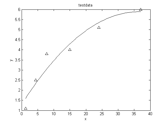
function plot_excel_data                        %  © J. M. Hill S2011
% read data from excel file into a matrix, plot designated columns as
% discrete points, overlay plot of curve fit
% user must edit code for correct values of filename, xcol, ycol, n
% and plot title and labels
clc;                %clear command window
filename = 'test.xlsx';
xcol = 2;           %column xcol in the a matrix will be read into vector x
ycol = 4;           %column ycol in the a matrix will be read into vector y
[x,y] = read_excel_cols(filename,xcol,ycol);  %read colmuns from excel file
plot_data(x,y)
%--------------------------------------------------------------------------
function [x,y] = read_excel_cols(filename, xcol, ycol)
c = xlsread(filename);  % read all the data in the file into array a
x = c(:,xcol);          % assign all numbers in col xcol to vector x
y = c(:,ycol);          % assign all numbers in col ycol to vector y
[n,m] = size(c);        %determine size, n rows, m columns
b = c(:,m);             %strip b vector out of c matrix
for i = 1:n
    for j = 1:n
        a(i,j) = c(i,j);%strip a matrix out of c matrix
    end
end                     %alternatively: a = c(:,1:n) can replace the loop;
write_matrix_screen(n,a,b)
%--------------------------------------------------------------------------
function write_matrix_screen(n,a,b)
for i = 1:n
    for j = 1:n
        fprintf(1,'%3.2g ',a(i,j)); %write coefficient matrix to screen
    end
    fprintf(1,'%3.2g\n',b(i));      %write right-hand-side vector to screen
end
%--------------------------------------------------------------------------
function plot_data(x,y) %plot x-y pairs, overlay plot of curve fit
plot(x,y,'k^')
hold on                     % overlay plots
n = 2;                      % order of polynomial regression (max = 3)
c = polyfit(x,y,n);         % fit x-y pairs with polynomial of order n
ypred = polyval(c,x);       % predictions
dev = y - mean(y);          % deviations - measure of spread
SST = sum(dev.^2);          % total variation to be accounted for
resid = y - ypred;          % residuals - measure of mismatch
SSE = sum(resid.^2);        % variation NOT accounted for
Rsq = 1 - SSE/SST;          % percent of error explained (r-squared)
fprintf(1,'r-squared = %g\n',Rsq)
for i = 1:n+1
    fprintf('c(%d)= %6.4g\n',i,c(i));  %print polynomial coefficients
end
m = numel(x);          %determine the number of elements in vector x
dx = (x(m)-x(1))/100;  %calculate a delta-x equal to (last_x - first_x)/100
xx = x(1):dx:x(m);     %divide x scale into 100 ptsto make a good plot
switch n
    case 1                                                %linear fit
        line = c(1).*xx + c(2);
    case 2                                                %second-order fit
        line = c(1).*xx.^2 + c(2).*xx + c(3);
    case 3                                                %cubic fit
        line = c(1).*xx.^3 + c(2).*xx.^2 + c(3).*xx + c(4);
    otherwise
        disp('Cannot do fit greater than 3 with this code');
end
plot(xx,line,'k')
ylabel('y')
xlabel('x')
title('testdata')
hold off                %quit overlaying plots
  6 1.2   5 1.1   1   1 NaN
  7 4.4   6 2.5   2   2 NaN
  6 7.8   8 3.8   3   3 NaN
  7  15   5   4   4   4 NaN
  6  24   3 5.1   5   5 NaN
  7  37   1   6   6   6 NaN
r-squared = 0.935904
c(1)= -0.003445
c(2)= 0.2515
c(3)=  1.296
