| |
GeoDesign
Tutorial 0A - Basic GIS
In this tutorial you will obtain GIS data, organize
it in ArcCatalog, and view both spatial and attribute data in ArcMap.
The purpose of this tutorial is mainly to introduce you to the programs
and interface of the ArcGIS platform.
PART A. DATA ACQUISITION
- The data you will be using in this exercise (also some other exercises) comes from the Washington State Geospatial Data Archive
(WAGDA). All the data can be accessed from our course website. In each of the tutorials on the course website, you will find a link allowing you to download all the tutorial data.
- Create a working directory (a folder) in My Documents and name it "exercise1". Download the following five datasets (click HERE) to this folder:
- Municipal Boundaries
- Building Outlines
- Parcel Boundaries....(Land Use)
- Street Network…
- Metro Bus Stops
- These files are zipped, so you'll need to unzip
them in Windows Explorer and click the Extract
button to place the uncompressed files in your working directory.
PART B. FILE ORGANIZATION
The first thing you'll need to do with ArcGIS is to use ArcCatalog
to establish a connection to your working directory. The ArcGIS
file system does not automatically provide access to the
full Windows file system, so whenever you start a new working directory,
you'll need to explicitly create a connection to it.
- In the Start menu, open the Programs
submenu, then choose the subdirectory ArcGIS
and select ArcCatalog.
- Once ArcCatalog has opened, find and click the Connect
to Folder button on the main toolbar:

- In the dialog box that appears, navigate to your working directory, then click OK.
- Now let's look at the ArcCatalog interface. The left portion
shows a directory tree, listing all connections that have been
made, all under the top-level directory called Catalog.
Notice that your working directory now appears in this directory
tree.
- Open your working directory by double-clicking on it, and inspect
its contents to be sure that all five of the layers you downloaded
have appeared. Notice that the five layers have three different
icons associated with them. The busstop layer's
icon indicates a point layer, the snd
layer's icon indicates a polyline layer, and
the icon next to boundary, parcel
and bldg indicates a polygon
layer.
The right portion of the ArcCatalog interface shows the contents,
preview, or metadata for whatever is currently selected in the
directory tree at the left. While your working directory is selected,
you should see the five layers you download, along with the type for each (they should all be Shapefiles). This area allows you
to quickly inspect data files one-by-one before adding them to
an ArcMap project.
- Now select the "snd" layer in your
directory tree. You'll see the right side change to a large icon
indicating this is a shapefile with polyline data. Click on the
Preview tab to look at the spatial data. You'll
now see a map of all of the principal transit routes in Seattle.
At the bottom of the preview, change the drop-down box from Geography
to Table and scroll across to see what kinds
of attribute data are included in this layer.
- Select "busstop" layer and repeat
the previous step. Question1: How
many bus stops can you find in the attribute table (look at table
record)?
PART C. VIEWING MAP DATA
Next, you will begin an ArcMap project. ArcMap is the program in
which you can view, edit, and manipulate spatial data layers in
detail, as well as prepare maps for output.
- Open ArcMap either through the Start menu or
by clicking on the Launch ArcMap button in ArcCatalog:

In the Getting Started dialog box, Choose Blank Map (the default option), then hit OK
- Now what you have is just an empty map, until you add DATA in
your map, ArcMap is not quite useful.
- Before you add data in, you have one thing to do: to tell ArcMap
to record only "relative path" to all the data sources
(as opposed to absolute path). Using relative paths allows you
to transfer your map between different computers without trouble,
especially when you plan to store your maps in a jump flash drive.
Different computer may designate a different drive locator (E:
or F: or G: and so on) to the jump drive. Now go to File
> Map Document Properties... , then in the dialog
window check Store relative path names to data
sources, click OK to close the
dialog window.
- Now you can go ahead to add all five of your data layers into
ArcMap, first click on the Add Data button in
the main toolbar:

- In the Look in drop-down box, navigate to the
connection to your working directory. Then highlight all five
of your data layers by clicking the first one, holding down the
Shift key, and clicking on the last one, then click Add.
You should now see how the spatial data layers are listed in both
the left and right portions of the ArcMap interface. At left you
see what is called the Table of Contents, which
is simlar to a map legend in that it lists the five layers and
shows the symbology used to represent each layer on the map. At
right, you see the map itself, with bus stops on top, transit
routes beneath them, and parcels, buildings, and boundaries in the background.
- Let's start navigating around Seattle now. Zoom in by first
clicking on the Zoom In tool:

then by clicking on the map and drawing a box around the area
you want to zoom in on. Try this by zooming in on the University
District (don't know where it is? Please Google-map University of Washington and get an idea about its location in relation to the city of Seattle, it is roughly in the center of the city).
- (Tip: if the map looks incomplete and you
can't find the U District, you may have interrupted ArcMap
by clicking on the map while it was still drawing. To refresh
the view, hit the F5 key on your keyboard
and wait for it to finish drawing.)
- You may notice that there are no buildings shown on the University
of Washington campus. If this is so, it is probably because of
the order of your layers in the Table of Contents. In the Table
of Contents, layers at the bottom of the list are drawn first,
then layers above are drawn on top, so the lowest layers can get
covered up by the higher layers. If the bldg
layer is at the bottom, click on it and drag it upward until a
black horizontal line appears just above the parcel
layer, then let go of the mouse button.
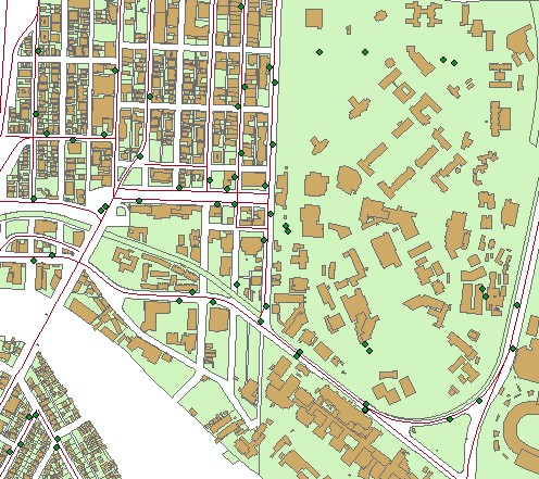
- You should now see building outlines of all of the campus buildings.
Continue zooming until you can tell where Gould Hall (or any building on campus) is but you
can still see its vicinity. You can continue to use the Zoom In
tool, but you may also need the Zoom Out tool
(
 )
to back out again or the Pan tool ( )
to back out again or the Pan tool ( )
to navigate laterally around the map. You should end up with a
view something like this (but your colors will differ): )
to navigate laterally around the map. You should end up with a
view something like this (but your colors will differ):
- Next, let's change the symbology of some of our layers. The
easiest way to change symbology is to simply click on the symbol
in the Table of Contents. Click on the symbol for the busstop
layer.
- You'll see a long list of basic symbols, but nothing particurly
good for bus stops. To add some options, click on the Style References... button, scroll down and check Civic. This
shows an entire new set of symbols added to the list.
- Scroll down to find the symbol called Bus 1.
Reduce the size from its default of 18 to a size of about 13.
Click OK to apply the new symbology.
- You can also apply symbology based on attributes of the features
shown in a layer. To try this, we will change the parcel symbology
to represent present-use categories for each parcel. right-click
on the parcel layer and select Properties....
- In the dialog box that appears, select the Symbology
tab. Under the Show list, select Categories
and leave the subtype as Unique values.
- Now, change the Value Field to PU_CAT_DES
in the drop-down list (it should be the last one).
- For now, you don't see any categories listed, so click on Add
All Values to get ArcMap to look through the data to
identify all of the categories of present use. Since you've included
all categories, you can un-check the checkbox next to <all
other values>.
- Select a color scheme you like by clicking on the drop-down
box under Color Scheme.
PART D. VIEWING ATTRIBUTE
DATA
As it happens, there is some more detailed present use information
in the parcel layer than what you see in the Table of Contents,
but it is a bit too detailed to be able to assign a different color
for each.
- To inspect this more detailed information, click on the Identify
button:

- With this tool, click on the Univerity of Washington campus.
This brings up the Identify Results box.
- First, make sure that the layer the data comes from is the parcel
layer by looking at the left side of this box. If it isn't, choose
parcel from the Layers drop-down
box and click again on the UW campus. You should now see a listing
of all data associated with this parcel.
- Question 2: What is the value
of the PRES_USE_D field? Is it at least a bit more detailed than
the PU_CAT_DES field?
- Another way to view a layer's attribute data is to open its
attribute table. This will display all data for all features in
a layer at the same time in a table format. To do this, right-click
on the parcel layer in the Table of Contents,
and select Open Attribute Table.
- Scroll across to see all of the attributes contained in the
parcel layer, and scroll down a bit to see what kinds of values
are taken on by these attributes. Some of these attributes are
spatial (such as area and perimeter),
but most of them are non-spatial, such as all of the present-use-related
fields.
- We can select a subset of the parcels by using these layer attributes.
Let's say we want to select all of the vacant parcels in Seattle.
To do this, click on the Options button at the
bottom of the attribute table, and select Select By Attributes....
- Find "PU_CAT_DES" in the Fields
list and double-click on it to put it in the query statement.
- Next, click (single-click) on the Like button to add the text-comparison
operator.
- In the Unique sample values list to the right,
find 'Vacant' and double-click on it. If you
don't see it in the list, click on the Get Unique Values
button to get ArcMap to search all records for all unique
values.
- After you've double-clicked on 'Vacant', you should see the
following in the query statement:
"PU_CAT_DES" LIKE 'Vacant'
If you don't, you can edit it directly to make sure it matches.
- Now click Apply, then Close
to close the query editor.
- In the Attribute Table, click the button Selected
to show only the records that have been selected. Now if you scroll
all the way to the right, you'll see that all of the records have
a "PU_CAT_DES" value of "Vacant". Question
3: How many vacant parcels you found? again look at records.
- Close the Attribute Table by clicking on its Close Box in its
upper-right-hand corner. You can now see that many of the parcels
in your view have been highlighted. These are the vacant parcels.
- When you're done looking at vacant parcels, you can choose the
menu item Selection > Clear Selected Features to
clear the selection.
PART E. MORE ABOUT SELECTING FEATURES
1. Download one more file by clicking HERE to your working directory:
- Capitol Hill & First Hill Urban Center (caphiluc)
2. add the data layer into ArcMap, using Add Data
button in the main toolbar
3. You already know you can select features By Attributes. You
can also select features by their location (their spatial relationship
to other features, whether in another layer or in the same layer).
To select features by location, the user specifies a selection method,
a selection layer, a spatial relationship, a reference layer, and
sometimes a distance buffer.
4. Let’s say you want to find out how many bus stops in the
Capitol Hill. Now you can use caphiluc polygon as your reference
layer to select bus stops in your selection layer, which is busstop
layer.
5. To begin selecting features by location, you click the Selection
menu and click the Select by Location option.
6. In the Select by Location dialog box, set all the options to
be read like the following: I want to select features from the following
layers busstop that intersect the features in this layer caphilus.
There are some graphics in preview showing you how features are
selected using this setting.
7. Now you should see all the bus stops within the district have
been highlighted. Then open the attribute table of busstop layer
and answer the following question. Question
4: How many bus stops you found in Capitol Hill? again look at records,
and show only selected.
8. When you're done looking at selected bus stops, you can choose
the menu item Selection > Clear Selected
Features to clear the selection.
PART F. CLIPPING FEATURES
Sometimes the acquired data sets cover a greater area than the
user is interested in. For example, all the layers you have downloaded
are for the entire Seattle area, but you might be only interested
in what is in Capitol Hill. The data set can be clipped to the area
of interest by using features in one layer to clip the features
in another layer. To do so, you will have to know about ArcToolbox.
ArcToolbox is the application that provides an
environment for performing geographic information system (GIS) analysis.
ArcToolbox allows the user to perform a variety
of geoprocessing tasks including data conversion. To access ArcToolbox,
click on the ArcToolbox icon in ArcMap.

To clip one layer based on another, the user must use Clip
found in the Extract portion of Analysis
Tools in ArcToolbox.
Now, for completing your exercise, you will have to
clip all the four layers: parcel, bldg, snd, and busstop,
for the area Capitol Hill.
In the Clip dialogue box, you choose,
each time, one of the four layers as the Input Features,
and choose the district boundary layer as the Clip Features,
and name your output layer (output feature class), or just use default
name, then you click OK to finish clipping. You
will see that the output layer will be added into your map.
PART G. CREATING MAPs
When you open ArcMap, you often view the data layer in Data
View. To view the data in layout view, which is
the view in which a map will be printed, the user must click on
the View menu and select Layout View.
Or Click on the small Layout View icon under your
map content window.
Map elements may be arranged within a variety of paper sizes. In
addition, the orientation of a page may be either horizontal or
vertical. It is recommended that the user specifies these characteristics
before they begin the map layout process.
Paper sizes and orientation can be selected by clicking on the File
menu and selecting Page and Print Setup. The Page
Setup dialog box will appear. For this exercise, use Letter
size.
A map title may be added to the layout by clicking
the Insert menu and selecting the Title option. A text box will
be added to the page. Within this text box, a default title will
be present. The user can type in a preferred title within the text
box and press Enter. After the Enter key has been pressed, the user
can go back and edit the title by double-clicking the on the title
and editing its text properties.
The font, size, style, or color of the title may be changed using
the Draw Toolbar.
A North Arrow may be added by clicking the Insert menu and selecting the North Arrow option. The user can resize the
north arrow by clicking and dragging on one of its corners. In addition,
the user can move the north arrow to any desired location within
the map layout.
Other elements may be added include: A Scale Bar,
texts, and A Legend. A Legend
may be added by clicking the Insert menu and selecting the Legend
option.
By default, the legend includes all layers from the map, and the
number of legend columns is set to one. The user can choose which
layers may be displayed in the legend by selecting the layer from
the Map Layer box and clicking the right arrow
(>>). The selected layers will be displayed
in the Legend Items box.
Now, to finish up this exercise,
please create two maps:
- One of which shows the entire Seattle with Capitol Hill being highlighted only.
- The other one shows only Capital Hill with streets, buildings, and Bus stops on the map.
To export your maps, go to File menu, (remember
you still in Layout View), and then Export Map,
choose .jpeg, or .tiff
as the image format, set image quality to high, navigate to your
working directory, finally save your maps as images.
Then, you can insert your maps in a Microsoft Word document.
The deliverable:
Submit your Word document with the two maps to Moodle before Sep 8, 5:00pm.
PART H. SAVING YOUR DATA
The last step in this process is to save your work. While the data
itself is already saved as shapefiles, you can also save your layout
and symbology as an ArcMap Project File (*.mxd).
- Click on the Save button:

- You will be promted to save your file in a location in the full
Windows file system. Find your working directory and save it there
as something like "Exercise1.mxd".
- When you've finished this, you should exit ArcMap and ArcCatalog,
then backup your ArcMap Project on a flash drive. You don't really
need to backup the Shapefiles, since they are too large to fit
them all on a flash drive, and you can always download them again
from the course website. If you do this, however, you'll need to be sure to
put the ArcMap Project file in the same place relative to the
data files, so that it can easily find them in the directory system.
Tutorial 0B - Linking External Data & Vector/Raster Conversion
PART A. SETTING UP THE PROJECT
- Download the following three datasets by clicking HERE and put them into your working directory in My Documents (remember
to unzip and extract them using Windows Explorer):
- Extent of Water Bodies and Land (sndshore)
- Metro Transit Revenue Service Routes (tpipath_rev_cur)
- Metro Transit Route Timepoints (timepoint)
- Open ArcMap and add all of the above datasets to a new project.
- Adjust the symbologies for easy viewing. Here are some suggestions:
- For the tpipath_rev_cur dataset, change the symbology to
a thin black line;
- For the sndshore dataset,
set the symbology using Categories: Unique Values,
using the field feature. This setting will display
each sndshore feature differently depending on what
its feature value is. To see a list of all of the
distinct feature values, click on the Add All Values button. For the feature "waterbody", set the symbology to
"Lake" (by double-clicking on the current symbol next to
"waterbody"). Lastly, remove the symbologies for "land"
and "mudholes" (by right-clicking on each one, in turn, and clicking
the Remove Value(s) button) and uncheck the box next to "<all
other values>".
PART B. LINKING EXTERNAL DATA
You are now going to import a non-spatial data table into ArcMap. The
table is a xls format file (MS Excel) with two columns. The first column lists
the time-point key for all of the transit route time points in the Metro
bus system. The second column lists the number of routes that use that
time point. We are going to use this as an indicator of the level of transit
coverage in different areas of the City of Seattle.
Note: I generated this table by a very simple process in SPSS of taking
the Metro transit pattern table (available in the Transportation subheading
of the King County part of WAGDA) and aggregating it by time-point key,
recording the number of rows that have each value of time-point key.
- Download a table containing the number of bus routes passing each
time point by clicking here.
- Add it into your ArcMap project. (select tpfreq$ table)
- At the top of the Table of Contents, click on Source tab, you will then see the table you just added in,
- Open the table by right-clicking on its name in the Table of Contents
and selecting Open.
- To get some information on the frequencies listed in this table, right-click
on the heading FREQUENC and click on Statistics.
How many different time points are represented in the table? What are
the minimum and maximum values in the field FREQUENC?
When you're done, click on the X-shaped close box in the upper right corner of the dialog box, then click on the close
box for the table itself.
- Now you will join this non-spatial table with a spatial dataset, the timepoint dataset, using the unique identifier for the
time point as the linking variable. In the Table of Contents, right-click
on the name of the timepoint dataset and select Joins
and Relates > Join....
- In the box that appears, change the following settings:
- Set the drop-down box under "1." to TIMEPT_ID.
- Set the drop-down box under "2." to tpfreq$.
- Set the drop-down box under "3." to KEYTMPT.
- Click the OK button.
- Now change the symbology for the timepoint dataset using the newly
attached data. Right-click on the name timepoint in the
Table of Contents and select Properties....
- Under the Symbology tab, change the type of sumbology
to Quantities > Graduated colors. Click on the drop-down
box next to Value. In the
drop-down box, find and select "FREQUENC". Right-click
on one of the symbols and select Properties for All Symbols.
In the Symbol Selector dialog box, click on the Edit Symbol... button and uncheck the checkbox next to Use Outline.
Click OK twice to get back to the Layer Properties.
Last, change the number of Classes to "32"
and click OK.
- Your map will look like this:
PART C. GENERATING A RASTER LAYER FROM POINT DATA
(For those who are still having trouble finishing this following step, please download the TRA raster layer by clicking this link. Please extract the layer to your folder and add it into your ArcMap file and continue to the next part.)
In this step, you will use the Time Points dataset to estimate a surface
that represents an abstract quantity we'll call "Transit Route Accessibility".
For short, let's call that abstract quantity "TRA". You will
do this by creating a raster layer that estimates the TRA value at every grid location, even when there is no Time Point at that location. The
procedure you will use does this by interpolating between Time Points
in the vicinity of each grid location on the raster dataset.
- First, make sure that Spatial Analyst is activated. You can go to Customize menu then select Extensions.., make sure the box next to Spatial Analyst is checked.
- Open ArcToolbox by clicking on the icon under the menu.
- In the ArcToolbox, click on the small "plus" (+) in front of Spatial Analyst Tools, then Interpolate, and double-click the
item IDW (which stands for Inverse Distance Weighted).
- In the dialog box that appears, set the following:
- Set Input Points to timepoint,
- Set Z value field to tpfreq$.FREQUENC,
- name your Output raster by clicking on the
open folder button, navigating to your personal directory, and giving the new raster dataset a name, such as "TRA".
- Set the Output cell size to 200
- Set Power to 2,
- Set Search radius type to variable,
- Set Number of points to 4 (and
leave blank the Maximum Distance),
- Click OK to start the operation. This may take a
minute to complete.
- The new raster dataset will automatically be inserted into your working
project. Double-click on its name to edit the symbology.
- Under the Symbology tab, change the Show type to Stretched.
- Change the color ramp to one of your liking. I'd suggest the one that
has yellow on the left and blue on the right, then clicking on the Invert checkbox to reverse the direction of the color ramp. When you're done,
click OK.
- Now navigate around the map of Seattle and think about the information
that is shown here.
- What areas of Seattle seem to have the greatest Transit Route
Accessibility?
PART D. CONVERTING A RASTER DATASET TO A VECTOR CONTOUR DATASET
In this part, you will create a vector dataset containing contour lines
generated from the raster dataset that you created in Part C.
- In the ArcToolbox, Go into the Spatial Analyst Tools again, this time
finding the submenu Surface Analysis and thec double-click the
item Contour....
- In the dialog that appears, set the following:
- Set Input surface to the name of your raster
dataset for Transit Route Accessibility (TRA),
- Set the Contour Interval to 10,
- Set the Base Contour to 0, and
- Set the Z Factor to 1.
Also name your Output features by clicking on the
open folder button, navigating to your personal directory, and giving the new feature dataset a name, such as "TRAcontour".
- Click OK to start the operation, which should be
completed in very little time.
- Now set the symbology for your new contour dataset by double-clicking
on its name in the Table of Contents.
- Under the Symbology tab, change the Show type to Quantities: Graduate colors.
- Under Fields, change the value to CONTOUR. Increase the Number of Classes to 11.
- Set the Color Ramp to one you like. I also suggest
increasing the widths of the contour lines by right-clicking on any
of the symbols and selecting Properties for All Symbols,
then increasing the Width to 3.
- Click OK to exit the contour dataset's properties.
- Now compare the data depicted by the contour map to the data depicted
by the raster layer.
- How would you compare the results of the contour layer, in comparison
with the raster layer?
PART E. REPORTING YOUR FINDINGS
Create two JPEGs showing the City of Seattle, with one showing the raster layer of Transit Route Accessibility (from
Part C) and the other showing the contour layer (from Part D). Both maps
should also show the tpipath_rev_cur (transit routes) layer, the timepoint (time
points) layer, and the SNDSHORE layer to help provide geographical context.
You can add other layers as you like to help show the context, but stay
away from polygon layers, since it will be difficult to show both the
raster layer and a polygon layer at the same time.
The deliverable:
Submit your Word document with the two maps to Moodle before Sep 8, 5:00pm.
prepared by Ming-Chun Lee, 08/24/2015
|